In this blog post, we will take the MLP architecture we have been developing and complexify it. Instead of just looking at the last 3 characters, we'll look at more characters. We'll also avoid feeding all this information into one layer and instead make the model deeper, allowing it to soak up the information more gradually. The architecture we will develop is very similar to the WaveNet paper: https://arxiv.org/pdf/1609.03499.
Starting Point: Basic MLP Architecture
Here is where we are coming from - the same architecture as last time with the MLP approach:
import torch
import torch.nn.functional as F
import matplotlib.pyplot as plt # for making figures
# %matplotlib inline # This is not needed in a script

# read in all the words
words = open('names.txt', 'r').read().splitlines()
print(len(words))
print(max(len(w) for w in words))
print(words[:8])

# build the vocabulary of characters and mappings to/from integers
chars = sorted(list(set(''.join(words))))
stoi = {s:i+1 for i,s in enumerate(chars)}
stoi['.'] = 0
itos = {i:s for s,i in stoi.items()}
vocab_size = len(itos)
print(itos)
print(vocab_size)

# shuffle up the words
import random
random.seed(42)
random.shuffle(words)

# build the dataset
block_size = 3 # context length: how many characters do we take to predict the next one?

def build_dataset(words):
  X, Y = [], []

  for w in words:
    context = [0] * block_size
    for ch in w + '.':
      ix = stoi[ch]
      X.append(context)
      Y.append(ix)
      context = context[1:] + [ix] # crop and append

  X = torch.tensor(X)
  Y = torch.tensor(Y)
  print(X.shape, Y.shape)
  return X, Y

n1 = int(0.8*len(words))
n2 = int(0.9*len(words))
Xtr,  Ytr  = build_dataset(words[:n1])     # 80%
Xdev, Ydev = build_dataset(words[n1:n2])   # 10%
Xte,  Yte  = build_dataset(words[n2:])     # 10%

for x,y in zip(Xtr[:20], Ytr[:20]):
  print(''.join(itos[ix.item()] for ix in x), '-->', itos[y.item()])

# Near copy paste of the layers we have developed in Part 3

# -----------------------------------------------------------------------------------------------
class Linear:

  def __init__(self, fan_in, fan_out, bias=True):
    self.weight = torch.randn((fan_in, fan_out)) / fan_in**0.5 # note: kaiming init
    self.bias = torch.zeros(fan_out) if bias else None

  def __call__(self, x):
    self.out = x @ self.weight
    if self.bias is not None:
      self.out += self.bias
    return self.out

  def parameters(self):
    return [self.weight] + ([] if self.bias is None else [self.bias])

# -----------------------------------------------------------------------------------------------
class BatchNorm1d:

  def __init__(self, dim, eps=1e-5, momentum=0.1):
    self.eps = eps
    self.momentum = momentum
    self.training = True
    # parameters (trained with backprop)
    self.gamma = torch.ones(dim)
    self.beta = torch.zeros(dim)
    # buffers (trained with a running 'momentum update')
    self.running_mean = torch.zeros(dim)
    self.running_var = torch.ones(dim)

  def __call__(self, x):
    # calculate the forward pass
    if self.training:
      xmean = x.mean(0, keepdim=True) # batch mean
      xvar = x.var(0, keepdim=True) # batch variance
    else:
      xmean = self.running_mean
      xvar = self.running_var
    xhat = (x - xmean) / torch.sqrt(xvar + self.eps) # normalize to unit variance
    self.out = self.gamma * xhat + self.beta
    # update the buffers
    if self.training:
      with torch.no_grad():
        self.running_mean = (1 - self.momentum) * self.running_mean + self.momentum * xmean
        self.running_var = (1 - self.momentum) * self.running_var + self.momentum * xvar
    return self.out

  def parameters(self):
    return [self.gamma, self.beta]

# -----------------------------------------------------------------------------------------------
class Tanh:
  def __call__(self, x):
    self.out = torch.tanh(x)
    return self.out
  def parameters(self):
    return []

torch.manual_seed(42); # seed rng for reproducibility

n_embd = 10 # the dimensionality of the character embedding vectors
n_hidden = 200 # the number of neurons in the hidden layer of the MLP

C = torch.rand((vocab_size, n_embd))
layers = [
    Linear(n_embd * block_size, n_hidden, bias=False), BatchNorm1d(n_hidden), Tanh(),
    Linear(n_hidden, vocab_size),
]

# parameter init
with torch.no_grad():
    layers[-1].weight *= 0.1 # last layer make less confident

parameters = [C] + [p for layer in layers for p in layer.parameters()]
print(sum(p.nelement() for p in parameters)) # number of parameters in total
for p in parameters:
    p.requires_grad = True

# same optimization as last time
max_steps = 200000
batch_size = 32
lossi = []

for i in range(max_steps):

  # minibatch construct
  ix = torch.randint(0, Xtr.shape[0], (batch_size,))
  Xb, Yb = Xtr[ix], Ytr[ix] # batch X,Y

  # forward pass
  emb = C[Xb] # embed the characters into vectors
  x = emb.view(emb.shape[0], -1) # concatenate the vectors
  for layer in layers:
    x = layer(x)
  loss = F.cross_entropy(x, Yb) # loss function

  # backward pass
  for p in parameters:
    p.grad = None
  loss.backward()

  # update
  lr = 0.1 if i < 150000 else 0.01 # step learning rate decay
  for p in parameters:
    p.data += -lr * p.grad

  # track stats
  if i % 10000 == 0: # print every once in a while
    print(f'{i:7d}/{max_steps:7d}: {loss.item():.4f}')
  lossi.append(loss.log10().item())

plt.plot(lossi)

# put layers into eval mode (needed for batchnorm especially)
for layer in layers:
  layer.training = False

@torch.no_grad() # this decorator disables gradient tracking
def split_loss(split):
  x,y = {
    'train': (Xtr, Ytr),
    'val': (Xdev, Ydev),
    'test': (Xte, Yte),
  }[split]
  emb = C[x] # (N, block_size, n_embd)
  x = emb.view(emb.shape[0], -1) # concat into (N, block_size * n_embd)
  for layer in layers:
    x = layer(x)
  loss = F.cross_entropy(x, y)
  print(split, loss.item())

# put layers into eval mode
for layer in layers:
  layer.training = False
split_loss('train')
split_loss('val')

for _ in range(20):

    out = []
    context = [0] * block_size # initialize with all ...
    while True:
      # forward pass the neural net
      emb = C[torch.tensor([context])] # (1,block_size,n_embd)
      x = emb.view(emb.shape[0], -1) # concatenate the vectors
      for layer in layers:
        x = layer(x)
      logits = x
      probs = F.softmax(logits, dim=1)
      # sample from the distribution
      ix = torch.multinomial(probs, num_samples=1).item()
      # shift the context window and track the samples
      context = context[1:] + [ix]
      out.append(ix)
      # if we sample the special '.' token, break
      if ix == 0:
        break

    print(''.join(itos[i] for i in out))
The losses from this baseline code are:
train: 2.055196523666382
val: 2.103283643722534
First Improvements
Let's make several improvements to our model. We'll create a better loss plot by averaging over 1000 datapoints. We'll PyTorchify the embeddings and Flatten layers instead of special casing them. Instead of using a raw list of layers, we'll use the Sequential class. Most importantly, we'll take 8 characters instead of just 3 for our context window.
Even with just this change to 8 characters, the performance impact is pretty noticeable. The improved losses are:
train: 1.9202139377593994
val: 2.030952215194702
Here is the code for these improvements:
# read in all the words
words = open('names.txt', 'r').read().splitlines()
print(len(words))
print(max(len(w) for w in words))
print(words[:8])

# build the vocabulary of characters and mappings to/from integers
chars = sorted(list(set(''.join(words))))
stoi = {s:i+1 for i,s in enumerate(chars)}
stoi['.'] = 0
itos = {i:s for s,i in stoi.items()}
vocab_size = len(itos)
print(itos)
print(vocab_size)

# shuffle up the words
import random
random.seed(42)
random.shuffle(words)

# build the dataset
block_size = 8 # context length: how many characters do we take to predict the next one?

def build_dataset(words):
  X, Y = [], []

  for w in words:
    context = [0] * block_size
    for ch in w + '.':
      ix = stoi[ch]
      X.append(context)
      Y.append(ix)
      context = context[1:] + [ix] # crop and append

  X = torch.tensor(X)
  Y = torch.tensor(Y)
  print(X.shape, Y.shape)
  return X, Y

n1 = int(0.8*len(words))
n2 = int(0.9*len(words))
Xtr,  Ytr  = build_dataset(words[:n1])     # 80%
Xdev, Ydev = build_dataset(words[n1:n2])   # 10%
Xte,  Yte  = build_dataset(words[n2:])     # 10%

for x,y in zip(Xtr[:20], Ytr[:20]):
  print(''.join(itos[ix.item()] for ix in x), '-->', itos[y.item()])

# Near copy paste of the layers we have developed in Part 3

# -----------------------------------------------------------------------------------------------
class Linear:

  def __init__(self, fan_in, fan_out, bias=True):
    self.weight = torch.randn((fan_in, fan_out)) / fan_in**0.5 # note: kaiming init
    self.bias = torch.zeros(fan_out) if bias else None

  def __call__(self, x):
    self.out = x @ self.weight
    if self.bias is not None:
      self.out += self.bias
    return self.out

  def parameters(self):
    return [self.weight] + ([] if self.bias is None else [self.bias])

# -----------------------------------------------------------------------------------------------
class BatchNorm1d:

  def __init__(self, dim, eps=1e-5, momentum=0.1):
    self.eps = eps
    self.momentum = momentum
    self.training = True
    # parameters (trained with backprop)
    self.gamma = torch.ones(dim)
    self.beta = torch.zeros(dim)
    # buffers (trained with a running 'momentum update')
    self.running_mean = torch.zeros(dim)
    self.running_var = torch.ones(dim)

  def __call__(self, x):
    # calculate the forward pass
    if self.training:
      xmean = x.mean(0, keepdim=True) # batch mean
      xvar = x.var(0, keepdim=True) # batch variance
    else:
      xmean = self.running_mean
      xvar = self.running_var
    xhat = (x - xmean) / torch.sqrt(xvar + self.eps) # normalize to unit variance
    self.out = self.gamma * xhat + self.beta
    # update the buffers
    if self.training:
      with torch.no_grad():
        self.running_mean = (1 - self.momentum) * self.running_mean + self.momentum * xmean
        self.running_var = (1 - self.momentum) * self.running_var + self.momentum * xvar
    return self.out

  def parameters(self):
    return [self.gamma, self.beta]

# -----------------------------------------------------------------------------------------------
class Tanh:
  def __call__(self, x):
    self.out = torch.tanh(x)
    return self.out
  def parameters(self):
    return []

# -----------------------------------------------------------------------------------------------
class Embedding:

  def __init__(self, num_embeddings, embedding_dim):
    self.weight = torch.randn((num_embeddings, embedding_dim))

  def __call__(self, IX):
    self.out = self.weight[IX]
    return self.out

  def parameters(self):
    return [self.weight]

# -----------------------------------------------------------------------------------------------
class Flatten:

  def __call__(self, x):
    self.out = x.view(x.shape[0], -1)
    return self.out

  def parameters(self):
    return []

# -----------------------------------------------------------------------------------------------

class Sequential:

  def __init__(self, layers):
    self.layers = layers

  def __call__(self, x):
    for layer in self.layers:
      x = layer(x)
    self.out = x
    return self.out

  def parameters(self):
    # get parameters of all layers and stretch them out into one list
    return [p for layer in self.layers for p in layer.parameters()]

torch.manual_seed(42); # seed rng for reproducibility

n_embd = 10 # the dimensionality of the character embedding vectors
n_hidden = 200 # the number of neurons in the hidden layer of the MLP

model = Sequential([
    Embedding(vocab_size, n_embd),
    Flatten(),
    Linear(n_embd * block_size, n_hidden, bias=False), BatchNorm1d(n_hidden), Tanh(),
    Linear(n_hidden, vocab_size),
])

# parameter init
with torch.no_grad():
    model.layers[-1].weight *= 0.1 # last layer make less confident

parameters = model.parameters()
print(sum(p.nelement() for p in parameters)) # number of parameters in total
for p in parameters:
    p.requires_grad = True

# same optimization as last time
max_steps = 200000
batch_size = 32
lossi = []

for i in range(max_steps):
    # minibatch construct
    ix = torch.randint(0, Xtr.shape[0], (batch_size,))
    Xb, Yb = Xtr[ix], Ytr[ix] # batch X,Y

    # forward pass
    logits = model(Xb)
    loss = F.cross_entropy(logits, Yb) # loss function

    # backward pass
    for p in parameters:
        p.grad = None
    loss.backward()

    # update
    lr = 0.1 if i < 150000 else 0.01 # step learning rate decay
    for p in parameters:
        p.data += -lr * p.grad

    # track stats
    if i % 10000 == 0: # print every once in a while
        print(f'{i:7d}/{max_steps:7d}: {loss.item():.4f}')
    lossi.append(loss.log10().item())

plt.plot(torch.tensor(lossi).view(-1, 1000).mean(1))

lossi[:10]

# put layers into eval mode (needed for batchnorm especially)
for layer in model.layers:
  layer.training = False

@torch.no_grad() # this decorator disables gradient tracking
def split_loss(split):
    x,y = {
    'train': (Xtr, Ytr),
    'val': (Xdev, Ydev),
    'test': (Xte, Yte),
    }[split]
    logits = model(x)
    loss = F.cross_entropy(logits, y)
    print(split, loss.item())

split_loss('train')
split_loss('val')

for _ in range(20):

    out = []
    context = [0] * block_size # initialize with all ...
    while True:
      # forward pass the neural net
        logits = model(torch.tensor([context]))
        probs = F.softmax(logits, dim=1)
        # sample from the distribution
        ix = torch.multinomial(probs, num_samples=1).item()
        # shift the context window and track the samples
        context = context[1:] + [ix]
        out.append(ix)
        # if we sample the special '.' token, break
        if ix == 0:
            break

    print(''.join(itos[i] for i in out))
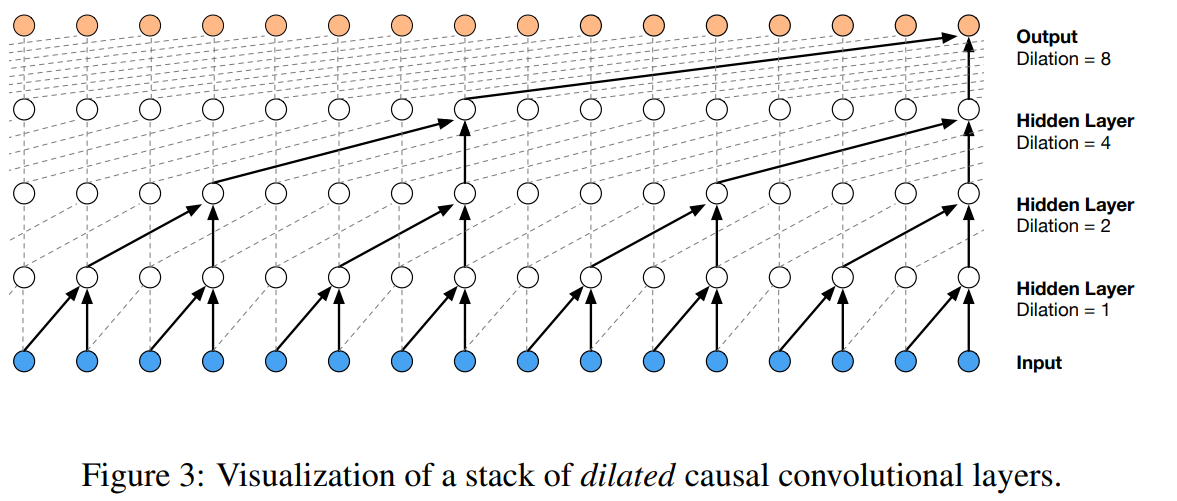
WaveNet-Inspired Architecture
Now let's change up the architecture to follow the WaveNet paper structure. We want to implement a hierarchical structure where adjacent pairs of characters are processed together before being combined.
Let's examine the shapes in our current model. If we have 4 examples in our batch with 8 characters per example, we start with shape (4, 8). After embedding each character into 10 dimensions, we get (4, 8, 10). We then flatten this to (4, 80) and feed it into the linear layer to get (4, 200).
In the current linear layer, we perform (4, 80) @ (80, 200) + 200. For each example, we have 10 numbers for character 1, 10 numbers for character 2, etc. We have something like positions 1, 2, 3, 4, 5, 6, 7, 8.
With the new WaveNet architecture, we want the first layer to process adjacent pairs: (1, 2), (3, 4), (5, 6), (7, 8). In code, we want to perform operations like (4, 4, 20) @ (20, 200) + 200. This essentially requires changing both the Flatten layer and the Linear layer's expected input size. The n_hidden parameter becomes 68 in this configuration.
The performance improvement isn't dramatic, but we also need to update our BatchNorm implementation. Previously, BatchNorm was only averaging over dimension 0, but now we will average over both dimensions 0 and 1.
Here is the implementation:
# read in all the words
words = open('names.txt', 'r').read().splitlines()
print(len(words))
print(max(len(w) for w in words))
print(words[:8])

# build the vocabulary of characters and mappings to/from integers
chars = sorted(list(set(''.join(words))))
stoi = {s:i+1 for i,s in enumerate(chars)}
stoi['.'] = 0
itos = {i:s for s,i in stoi.items()}
vocab_size = len(itos)
print(itos)
print(vocab_size)

# shuffle up the words
import random
random.seed(42)
random.shuffle(words)

# build the dataset
block_size = 8 # context length: how many characters do we take to predict the next one?

def build_dataset(words):
  X, Y = [], []

  for w in words:
    context = [0] * block_size
    for ch in w + '.':
      ix = stoi[ch]
      X.append(context)
      Y.append(ix)
      context = context[1:] + [ix] # crop and append

  X = torch.tensor(X)
  Y = torch.tensor(Y)
  print(X.shape, Y.shape)
  return X, Y

n1 = int(0.8*len(words))
n2 = int(0.9*len(words))
Xtr,  Ytr  = build_dataset(words[:n1])     # 80%
Xdev, Ydev = build_dataset(words[n1:n2])   # 10%
Xte,  Yte  = build_dataset(words[n2:])     # 10%

for x,y in zip(Xtr[:20], Ytr[:20]):
  print(''.join(itos[ix.item()] for ix in x), '-->', itos[y.item()])

# Near copy paste of the layers we have developed in Part 3

# -----------------------------------------------------------------------------------------------
class Linear:

  def __init__(self, fan_in, fan_out, bias=True):
    self.weight = torch.randn((fan_in, fan_out)) / fan_in**0.5 # note: kaiming init
    self.bias = torch.zeros(fan_out) if bias else None

  def __call__(self, x):
    self.out = x @ self.weight
    if self.bias is not None:
      self.out += self.bias
    return self.out

  def parameters(self):
    return [self.weight] + ([] if self.bias is None else [self.bias])

# -----------------------------------------------------------------------------------------------
class BatchNorm1d:

  def __init__(self, dim, eps=1e-5, momentum=0.1):
    self.eps = eps
    self.momentum = momentum
    self.training = True
    # parameters (trained with backprop)
    self.gamma = torch.ones(dim)
    self.beta = torch.zeros(dim)
    # buffers (trained with a running 'momentum update')
    self.running_mean = torch.zeros(dim)
    self.running_var = torch.ones(dim)

  def __call__(self, x):
    # calculate the forward pass
    if self.training:
      xmean = x.mean(0, keepdim=True) # batch mean
      xvar = x.var(0, keepdim=True) # batch variance
    else:
      xmean = self.running_mean
      xvar = self.running_var
    xhat = (x - xmean) / torch.sqrt(xvar + self.eps) # normalize to unit variance
    self.out = self.gamma * xhat + self.beta
    # update the buffers
    if self.training:
      with torch.no_grad():
        self.running_mean = (1 - self.momentum) * self.running_mean + self.momentum * xmean
        self.running_var = (1 - self.momentum) * self.running_var + self.momentum * xvar
    return self.out

  def parameters(self):
    return [self.gamma, self.beta]

# -----------------------------------------------------------------------------------------------
class Tanh:
  def __call__(self, x):
    self.out = torch.tanh(x)
    return self.out
  def parameters(self):
    return []

# -----------------------------------------------------------------------------------------------
class Embedding:

  def __init__(self, num_embeddings, embedding_dim):
    self.weight = torch.randn((num_embeddings, embedding_dim))

  def __call__(self, IX):
    self.out = self.weight[IX]
    return self.out

  def parameters(self):
    return [self.weight]

# -----------------------------------------------------------------------------------------------
class Flatten:

  def __call__(self, x):
    self.out = x.view(x.shape[0], -1)
    return self.out

  def parameters(self):
    return []

# -----------------------------------------------------------------------------------------------

class Sequential:

  def __init__(self, layers):
    self.layers = layers

  def __call__(self, x):
    for layer in self.layers:
      x = layer(x)
    self.out = x
    return self.out

  def parameters(self):
    # get parameters of all layers and stretch them out into one list
    return [p for layer in self.layers for p in layer.parameters()]

torch.manual_seed(42); # seed rng for reproducibility

n_embd = 10 # the dimensionality of the character embedding vectors
n_hidden = 200 # the number of neurons in the hidden layer of the MLP

model = Sequential([
    Embedding(vocab_size, n_embd),
    Flatten(),
    Linear(n_embd * block_size, n_hidden, bias=False), BatchNorm1d(n_hidden), Tanh(),
    Linear(n_hidden, vocab_size),
])

# parameter init
with torch.no_grad():
    model.layers[-1].weight *= 0.1 # last layer make less confident

parameters = model.parameters()
print(sum(p.nelement() for p in parameters)) # number of parameters in total
for p in parameters:
    p.requires_grad = True

# same optimization as last time
max_steps = 200000
batch_size = 32
lossi = []

for i in range(max_steps):
    # minibatch construct
    ix = torch.randint(0, Xtr.shape[0], (batch_size,))
    Xb, Yb = Xtr[ix], Ytr[ix] # batch X,Y

    # forward pass
    logits = model(Xb)
    loss = F.cross_entropy(logits, Yb) # loss function

    # backward pass
    for p in parameters:
        p.grad = None
    loss.backward()

    # update
    lr = 0.1 if i < 150000 else 0.01 # step learning rate decay
    for p in parameters:
        p.data += -lr * p.grad

    # track stats
    if i % 10000 == 0: # print every once in a while
        print(f'{i:7d}/{max_steps:7d}: {loss.item():.4f}')
    lossi.append(loss.log10().item())

plt.plot(torch.tensor(lossi).view(-1, 1000).mean(1))

lossi[:10]

# put layers into eval mode (needed for batchnorm especially)
for layer in model.layers:
  layer.training = False

@torch.no_grad() # this decorator disables gradient tracking
def split_loss(split):
    x,y = {
    'train': (Xtr, Ytr),
    'val': (Xdev, Ydev),
    'test': (Xte, Yte),
    }[split]
    logits = model(x)
    loss = F.cross_entropy(logits, y)
    print(split, loss.item())

split_loss('train')
split_loss('val')

for _ in range(20):

    out = []
    context = [0] * block_size # initialize with all ...
    while True:
      # forward pass the neural net
        logits = model(torch.tensor([context]))
        probs = F.softmax(logits, dim=1)
        # sample from the distribution
        ix = torch.multinomial(probs, num_samples=1).item()
        # shift the context window and track the samples
        context = context[1:] + [ix]
        out.append(ix)
        # if we sample the special '.' token, break
        if ix == 0:
            break

    print(''.join(itos[i] for i in out))
With the new model structure modeling after the WaveNet paper and fixing the BatchNorm to sum over the batch dimensions (not just the 0th dimension), our losses are:
train: 1.9112857580184937
val: 2.0208795070648193
Key Observations and Lessons Learned
This experiment was admittedly not very structured - we were essentially taking shots in the dark with the hyperparameters. Each iteration is taking much longer now, and we don't have an experimental harness to properly tune these parameters.
We have successfully implemented a structure similar to the WaveNet paper, though we're missing some key components like the gating layer and proper convolutions. This gives us a hint about how this code relates to CNNs.
Convolutions in neural networks are primarily about efficiency. They allow you to slide the model over inputs and enable parallelization not in Python but in CUDA kernels. The dilated causal convolutional layers in WaveNet allow for a sort of data reuse, or a type of dynamic programming, to efficiently process multiple examples at once.
Development Process Insights
An important takeaway from this exercise is understanding the typical development process for building deep neural networks:
- Spend significant time in PyTorch documentation, understanding the shapes of inputs and the input/output specifications of each layer.
- Work extensively on making shapes compatible, involving lots of permuting and viewing operations.
- Prototype these layers in Jupyter notebooks to ensure the shapes work correctly.
- Once satisfied with the prototypes, copy and paste the working code into a proper development environment like VSCode.
This process of reimplementing torch.nn modules from scratch unlocks many future directions. Moving forward, we can leverage the full power of torch.nn while understanding what's happening under the hood.
Future Directions
This foundation opens up several exciting areas for exploration:
- Implementing dilated causal convolutions from the WaveNet paper
- Understanding residual connections and skip connections and why they are useful
- Developing a proper experimental harness for systematic hyperparameter tuning
- Covering RNNs and LSTMs
- Building more sophisticated architectures
The key insight is that while we can now use torch.nn for efficiency, understanding the underlying implementations helps us make better architectural decisions and debug issues when they arise.