In our previous work with micrograd, we created an autograd engine based on scalars. However, PyTorch's autograd engine operates at the tensor level. As Andrej Karpathy says, "loss.backward()" is a leaky abstraction - not fully understanding how the backward pass works when finding the loss with respect to each parameter can lead to bugs. Let's explore how to find the gradients of the loss with respect to each parameter manually, working at the tensor level.
Setting Up Our Neural Network
We start by building a character-level language model using a dataset of names. Our code reads in all the words from a names file and creates a vocabulary of characters with mappings to and from integers.
import torch
import torch.nn.functional as F
import matplotlib.pyplot as plt # for making figures
%matplotlib inline

# read in all the words
words = open('names.txt', 'r').read().splitlines()
print(len(words))
print(max(len(w) for w in words))
print(words[:8])
32033
15
['emma', 'olivia', 'ava', 'isabella', 'sophia', 'charlotte', 'mia', 'amelia']
Next, we build the vocabulary of characters and create mappings between characters and integers.
# build the vocabulary of characters and mappings to/from integers
chars = sorted(list(set(''.join(words))))
stoi = {s:i+1 for i,s in enumerate(chars)}
stoi['.'] = 0
itos = {i:s for s,i in stoi.items()}
vocab_size = len(itos)
print(itos)
print(vocab_size)
{1: 'a', 2: 'b', 3: 'c', 4: 'd', 5: 'e', 6: 'f', 7: 'g', 8: 'h', 9: 'i', 10: 'j', 11: 'k', 12: 'l', 13: 'm', 14: 'n', 15: 'o', 16: 'p', 17: 'q', 18: 'r', 19: 's', 20: 't', 21: 'u', 22: 'v', 23: 'w', 24: 'x', 25: 'y', 26: 'z', 0: '.'}
27
Building the Dataset
We use a context length of 3 characters to predict the next character in the sequence. The build_dataset function creates input-output pairs where X contains the context and Y contains the target character.
# build the dataset
block_size = 3 # context length: how many characters do we take to predict the next one?

def build_dataset(words):
  X, Y = [], []

  for w in words:
    context = [0] * block_size
    for ch in w + '.':
      ix = stoi[ch]
      X.append(context)
      Y.append(ix)
      context = context[1:] + [ix] # crop and append

  X = torch.tensor(X)
  Y = torch.tensor(Y)
  print(X.shape, Y.shape)
  return X, Y

import random
random.seed(42)
random.shuffle(words)
n1 = int(0.8*len(words))
n2 = int(0.9*len(words))

Xtr,  Ytr  = build_dataset(words[:n1])     # 80%
Xdev, Ydev = build_dataset(words[n1:n2])   # 10%
Xte,  Yte  = build_dataset(words[n2:])     # 10%
torch.Size([182625, 3]) torch.Size([182625])
torch.Size([22655, 3]) torch.Size([22655])
torch.Size([22866, 3]) torch.Size([22866])
Comparing Manual Gradients with PyTorch
We introduce a comparison function that will help us verify our manually calculated gradients against PyTorch's automatic gradients. This function checks for exact matches and approximate matches, reporting the maximum difference between our calculations and PyTorch's.
def cmp(s, dt, t):
  ex = torch.all(dt == t.grad).item()
  app = torch.allclose(dt, t.grad)
  maxdiff = (dt - t.grad).abs().max().item()
  print(f'{s:15s} | exact: {str(ex):5s} | approximate: {str(app):5s} | maxdiff: {maxdiff}')
Neural Network Architecture
Our neural network consists of an embedding layer, a hidden layer with batch normalization, and an output layer. We initialize all parameters with specific random seeds for reproducibility.
n_embd = 10 # the dimensionality of the character embedding vectors
n_hidden = 64 # the number of neurons in the hidden layer of the MLP

g = torch.Generator().manual_seed(2147483647) # for reproducibility
C  = torch.randn((vocab_size, n_embd),            generator=g)
# Layer 1
W1 = torch.randn((n_embd * block_size, n_hidden), generator=g) * (5/3)/((n_embd * block_size)**0.5)
b1 = torch.randn(n_hidden,                        generator=g) * 0.1 # using b1 just for fun, it's useless because of BN
# Layer 2
W2 = torch.randn((n_hidden, vocab_size),          generator=g) * 0.1
b2 = torch.randn(vocab_size,                      generator=g) * 0.1
# BatchNorm parameters
bngain = torch.randn((1, n_hidden))*0.1 + 1.0
bnbias = torch.randn((1, n_hidden))*0.1

parameters = [C, W1, b1, W2, b2, bngain, bnbias]
print(sum(p.nelement() for p in parameters)) # number of parameters in total
for p in parameters:
  p.requires_grad = True
4137Forward Pass Implementation
We implement the forward pass by breaking it down into smaller, manageable steps. Each step can be backpropagated through individually, making it easier to understand and debug.
batch_size = 32
n = batch_size # a shorter variable also, for convenience
# construct a minibatch
ix = torch.randint(0, Xtr.shape[0], (batch_size,), generator=g)
Xb, Yb = Xtr[ix], Ytr[ix] # batch X,Y

# forward pass, "chunkated" into smaller steps that are possible to backward one at a time

emb = C[Xb] # embed the characters into vectors
embcat = emb.view(emb.shape[0], -1) # concatenate the vectors
# Linear layer 1
hprebn = embcat @ W1 + b1 # hidden layer pre-activation
# BatchNorm layer
bnmeani = 1/n*hprebn.sum(0, keepdim=True)
bndiff = hprebn - bnmeani
bndiff2 = bndiff**2
bnvar = 1/(n-1)*(bndiff2).sum(0, keepdim=True) # note: Bessel's correction (dividing by n-1, not n)
bnvar_inv = (bnvar + 1e-5)**-0.5
bnraw = bndiff * bnvar_inv
hpreact = bngain * bnraw + bnbias
# Non-linearity
h = torch.tanh(hpreact) # hidden layer
# Linear layer 2
logits = h @ W2 + b2 # output layer
# cross entropy loss (same as F.cross_entropy(logits, Yb))
logit_maxes = logits.max(1, keepdim=True).values
norm_logits = logits - logit_maxes # subtract max for numerical stability
counts = norm_logits.exp()
counts_sum = counts.sum(1, keepdims=True)
counts_sum_inv = counts_sum**-1 # if I use (1.0 / counts_sum) instead then I can't get backprop to be bit exact...
probs = counts * counts_sum_inv
logprobs = probs.log()
loss = -logprobs[range(n), Yb].mean()

# PyTorch backward pass
for p in parameters:
  p.grad = None
for t in [logprobs, probs, counts, counts_sum, counts_sum_inv, # afaik there is no cleaner way
          norm_logits, logit_maxes, logits, h, hpreact, bnraw,
         bnvar_inv, bnvar, bndiff2, bndiff, hprebn, bnmeani,
         embcat, emb]:
  t.retain_grad()
loss.backward()
loss
Notice how this forward pass is much more granular than what we typically see. This granular approach allows us to examine the gradients of the loss with respect to each intermediate computation step.
Manual Backpropagation Implementation
Now we implement the backward pass manually, calculating gradients step by step using the chain rule. We work backwards from the loss to each parameter.
# as they are defined in the forward pass above, one by one

dlogprobs = torch.zeros_like(logprobs)
dlogprobs[range(n), Yb] = -1.0 / n
dprobs = (1 / probs) *  dlogprobs # boosting gradient
dcounts_sum_inv = (counts * dprobs).sum(1, keepdims=True)
dcounts = (counts_sum_inv * dprobs)
dcounts_sum = -1 * (counts_sum**-2)  *  dcounts_sum_inv
dcounts += (torch.ones_like(norm_logits) * dcounts_sum)
dnorm_logits = counts * dcounts
dlogits = dnorm_logits.clone() # clone for safety, will need to add later
dlogit_maxes = (-1 * dnorm_logits).sum(1, keepdims=True) # should be 0, because we are only using dlogits_maxes for numerical stability, it doesn't contribute anything to the loss
dlogits += F.one_hot(logits.max(1).indices, num_classes=logits.shape[1]) * dlogit_maxes # (32 * 27) * (32 * 1)
dh = dlogits @ W2.T
dW2 = h.T @ dlogits
db2 = dlogits.sum(0) # by default it throws out the empty dimension
dhpreact = (1.0 - h**2) * dh # remember the derivative formula from micrograd!
dbngain = (bnraw * dhpreact).sum(0, keepdims=True)
dbnraw = bngain * dhpreact
dbnbias = dhpreact.sum(0, keepdims=True)
dbnvar_inv = (bndiff * dbnraw).sum(0, keepdims=True)
dbndiff = bnvar_inv * dbnraw
dbnvar = -0.5 *((bnvar + 1e-5) ** -1.5)* dbnvar_inv
dbndiff2 = (1.0/(n-1)) * torch.ones_like(bndiff2) * dbnvar
dbndiff += (2 * bndiff) * dbndiff2
dhprebn = dbndiff.clone()
dbnmeani = (-1 * dbndiff).sum(0, keepdims=True)
dhprebn += 1.0/n * (torch.ones_like(hprebn) * dbnmeani)
dembcat = dhprebn @ W1.T
dW1 = embcat.T @ dhprebn
db1 = dhprebn.sum(0)
demb = dembcat.view(emb.shape)
dC = torch.zeros_like(C)
for r in range(emb.shape[0]):
    for c in range(emb.shape[1]):
        dC[Xb[r][c]] += demb[r][c]
Understanding Backpropagation Through Linear Layers
Before verifying our gradients, let's understand the process of finding gradients with respect to each parameter. This process is similar to our micrograd implementation, using the chain rule to find the gradient of the loss with respect to node x by multiplying the gradient of the immediate output of x with respect to the input of x. Like in micrograd, we add the contributions of gradients when the output of node x goes to multiple output nodes.
However, there are some key differences when working with tensors, particularly regarding the shapes of the tensors. Let's examine how to backpropagate through a linear layer with the forward pass O = a @ b + c.
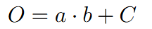
Here are the shapes of matrices a, b, c, O, and dO where dO represents the gradients of the loss with respect to O:
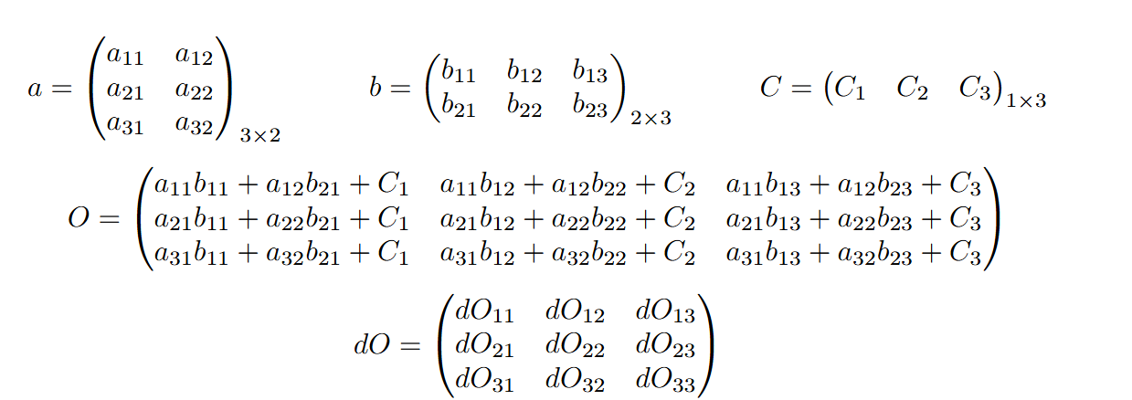
We want to calculate da, db, and dc, which are the gradients of the loss with respect to each of these matrices.
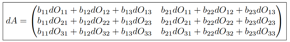
When determining what dA should be, dA must have the same shape as a. To find the values of da, we examine each cell of the O matrix, find where the corresponding cell of the a matrix is used, calculate the local gradient of that cell of a multiplied by the corresponding dO cell where the a value was used, and sum up all such contributions. For example, to find da_11, we find where a_11 is used (three times in the top three cells of dO), then sum up the contributions where each contribution is the local gradient times the loss with respect to the output. So da_11 would be b_11*dO_11 + b_12*dO_12 + b_13*dO_13.
Here is what da would be if you go through this process for all 6 cells:
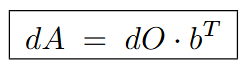
Which is equivalent to:
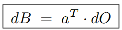
Similarly, we can go through this process to calculate dB and we get the following values:

Which is equivalent to:
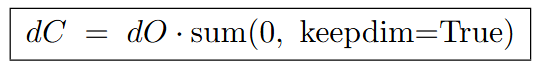
dC is slightly different. When we examine the values of O after computing a @ b + c, we see that values of C1, C2, and C3 are used in each cell of the 1st, 2nd, and 3rd columns respectively. Because they are only added and not multiplied by any other scalar, the derivative of the loss with respect to C is:

In PyTorch, we can write this as:
Verifying Our Manual Gradients
Let's check if our manually calculated gradients are close to what PyTorch calculated:
cmp('logprobs', dlogprobs, logprobs)
cmp('probs', dprobs, probs)
cmp('counts_sum_inv', dcounts_sum_inv, counts_sum_inv)
cmp('counts_sum', dcounts_sum, counts_sum)
cmp('counts', dcounts, counts)
cmp('norm_logits', dnorm_logits, norm_logits)
cmp('logit_maxes', dlogit_maxes, logit_maxes)
cmp('logits', dlogits, logits)
cmp('h', dh, h)
cmp('W2', dW2, W2)
cmp('b2', db2, b2)
cmp('hpreact', dhpreact, hpreact)
cmp('bngain', dbngain, bngain)
cmp('bnbias', dbnbias, bnbias)
cmp('bnraw', dbnraw, bnraw)
cmp('bnvar_inv', dbnvar_inv, bnvar_inv)
cmp('bnvar', dbnvar, bnvar)
cmp('bndiff2', dbndiff2, bndiff2)
cmp('bndiff', dbndiff, bndiff)
cmp('bnmeani', dbnmeani, bnmeani)
cmp('hprebn', dhprebn, hprebn)
cmp('embcat', dembcat, embcat)
cmp('W1', dW1, W1)
cmp('b1', db1, b1)
cmp('emb', demb, emb)
cmp('C', dC, C)
Excellent! We are correct!
Optimization 1: Logits to Loss Backpropagation
We can optimize our backpropagation calculations, particularly for the logits to loss computation and the batch normalization layers. Here's the optimization for the logits to loss backpropagation:
Before:
# dlogprobs = torch.zeros_like(logprobs)
# dlogprobs[range(n), Yb] = -1.0 / n
# dprobs = (1 / probs) *  dlogprobs # boosting gradient
# dcounts_sum_inv = (counts * dprobs).sum(1, keepdims=True)
# dcounts = (counts_sum_inv * dprobs)
# dcounts_sum = -1 * (counts_sum**-2)  *  dcounts_sum_inv
# dcounts += (torch.ones_like(norm_logits) * dcounts_sum)
# dnorm_logits = counts * dcounts
# dlogits = dnorm_logits.clone() # clone for safety, will need to add later
# dlogit_maxes = (-1 * dnorm_logits).sum(1, keepdims=True) # should be 0, because we are only using dlogits_maxes for numerical stability, it doesn't contribute anything to the loss
# dlogits += F.one_hot(logits.max(1).indices, num_classes=logits.shape[1]) * dlogit_maxes # (32 * 27) * (32 * 1)
After:
# backward pass
dlogits = F.softmax(logits, 1) # find probs along rows
dlogits[torch.arange(n), Yb] -= 1
dlogits /= n

cmp('logits', dlogits, logits) # I can only get approximate to be true, my maxdiff is 6e-9
logits | exact: False | approximate: True | maxdiff: 6.984919309616089e-09Let's understand what the gradients of the logits look like. We have 32 examples of 27 characters, where black squares indicate the correct characters.
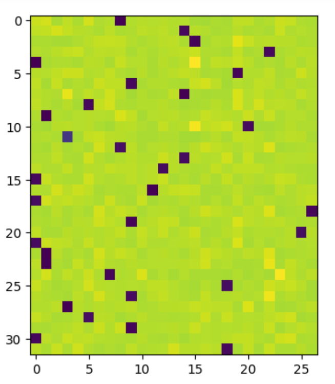
Intuitively, we are pulling down on the wrong characters and pulling up on the correct characters. The amount we push down on incorrect characters and push up on correct characters is the same - the sum of dlogits for each row is 0.
Optimization 2: BatchNorm Backpropagation
Here's the optimization for batch normalization backpropagation:
Before:
# dbnraw = bngain * dhpreact
# dbndiff = bnvar_inv * dbnraw
# dbnvar_inv = (bndiff * dbnraw).sum(0, keepdim=True)
# dbnvar = (-0.5*(bnvar + 1e-5)**-1.5) * dbnvar_inv
# dbndiff2 = (1.0/(n-1))*torch.ones_like(bndiff2) * dbnvar
# dbndiff += (2*bndiff) * dbndiff2
# dhprebn = dbndiff.clone()
# dbnmeani = (-dbndiff).sum(0)
# dhprebn += 1.0/n * (torch.ones_like(hprebn) * dbnmeani)
After:
# calculate dhprebn given dhpreact (i.e. backprop through the batchnorm)
# (you'll also need to use some of the variables from the forward pass up above)

dhprebn = bngain*bnvar_inv/n * (n*dhpreact - dhpreact.sum(0) - n/(n-1)*bnraw*(dhpreact*bnraw).sum(0))

cmp('hprebn', dhprebn, hprebn) # I can only get approximate to be true, my maxdiff is 9e-10
hprebn | exact: False | approximate: True | maxdiff: 9.313225746154785e-10Complete Training with Manual Backpropagation
Now let's put everything together and train the MLP neural network using our manual backward pass with the two optimizations:
# Exercise 4: putting it all together!
# Train the MLP neural net with your own backward pass

# init
n_embd = 10 # the dimensionality of the character embedding vectors
n_hidden = 200 # the number of neurons in the hidden layer of the MLP

g = torch.Generator().manual_seed(2147483647) # for reproducibility
C  = torch.randn((vocab_size, n_embd),            generator=g)
# Layer 1
W1 = torch.randn((n_embd * block_size, n_hidden), generator=g) * (5/3)/((n_embd * block_size)**0.5)
b1 = torch.randn(n_hidden,                        generator=g) * 0.1
# Layer 2
W2 = torch.randn((n_hidden, vocab_size),          generator=g) * 0.1
b2 = torch.randn(vocab_size,                      generator=g) * 0.1
# BatchNorm parameters
bngain = torch.randn((1, n_hidden))*0.1 + 1.0
bnbias = torch.randn((1, n_hidden))*0.1

parameters = [C, W1, b1, W2, b2, bngain, bnbias]

print(sum(p.nelement() for p in parameters)) # number of parameters in total

# same optimization as last time
max_steps = 200000
batch_size = 32
n = batch_size # convenience
lossi = []

# use this context manager for efficiency once your backward pass is written (TODO)
with torch.no_grad():

  # kick off optimization
  for i in range(max_steps):

    # minibatch construct
    ix = torch.randint(0, Xtr.shape[0], (batch_size,), generator=g)
    Xb, Yb = Xtr[ix], Ytr[ix] # batch X,Y

    # forward pass
    emb = C[Xb] # embed the characters into vectors
    embcat = emb.view(emb.shape[0], -1) # concatenate the vectors
    # Linear layer
    hprebn = embcat @ W1 + b1 # hidden layer pre-activation
    # BatchNorm layer
    # -------------------------------------------------------------
    bnmean = hprebn.mean(0, keepdim=True)
    bnvar = hprebn.var(0, keepdim=True, unbiased=True)
    bnvar_inv = (bnvar + 1e-5)**-0.5
    bnraw = (hprebn - bnmean) * bnvar_inv
    hpreact = bngain * bnraw + bnbias
    # -------------------------------------------------------------
    # Non-linearity
    h = torch.tanh(hpreact) # hidden layer
    logits = h @ W2 + b2 # output layer
    loss = F.cross_entropy(logits, Yb) # loss function

    # backward pass
    for p in parameters:
      p.grad = None

    # manual backprop! #swole_doge_meme
    # -----------------

    # loss to logits
    dlogits = F.softmax(logits, 1) # find probs along rows
    dlogits[torch.arange(n), Yb] -= 1
    dlogits /= n

    # to second layer
    dh = dlogits @ W2.T
    dW2 = h.T @ dlogits
    db2 = dlogits.sum(0) # by default it throws out the empty dimension

    # tanh layer backprop
    dhpreact = (1.0 - h**2) * dh # remember the derivative formula from micrograd!

    # batchnorm backprop
    dbngain = (bnraw * dhpreact).sum(0, keepdims=True)
    dbnbias = dhpreact.sum(0, keepdims=True)
    dhprebn = bngain*bnvar_inv/n * (n*dhpreact - dhpreact.sum(0) - n/(n-1)*bnraw*(dhpreact*bnraw).sum(0))

    # 1st layer
    dembcat = dhprebn @ W1.T
    dW1 = embcat.T @ dhprebn
    db1 = dhprebn.sum(0)

    # embeddings
    demb = dembcat.view(emb.shape)
    dC = torch.zeros_like(C)
    for r in range(emb.shape[0]):
        for c in range(emb.shape[1]):
            dC[Xb[r][c]] += demb[r][c]

    grads = [dC, dW1, db1, dW2, db2, dbngain, dbnbias]

    # -----------------

    # update
    lr = 0.1 if i < 100000 else 0.01 # step learning rate decay
    for p, grad in zip(parameters, grads):
      p.data += -lr * grad # new way of swole doge

    # track stats
    if i % 10000 == 0: # print every once in a while
      print(f'{i:7d}/{max_steps:7d}: {loss.item():.4f}')
    lossi.append(loss.log10().item())
Here is the output of the losses during training:
12297
   0/ 200000: 3.7932
10000/ 200000: 2.2055
20000/ 200000: 2.3798
30000/ 200000: 2.4544
40000/ 200000: 1.9862
50000/ 200000: 2.3561
60000/ 200000: 2.3519
70000/ 200000: 2.0542
80000/ 200000: 2.3711
90000/ 200000: 2.1424
100000/ 200000: 1.9349
110000/ 200000: 2.2606
120000/ 200000: 1.9823
130000/ 200000: 2.3847
140000/ 200000: 2.2810
150000/ 200000: 2.1436
160000/ 200000: 1.9847
170000/ 200000: 1.7666
180000/ 200000: 1.9904
190000/ 200000: 1.9243
Final Verification
Let's verify that the gradients we calculate align with PyTorch's calculated gradients for a few iterations:
# useful for checking your gradients
for p,g in zip(parameters, grads):
  cmp(str(tuple(p.shape)), g, p)
(27, 10)        | exact: False | approximate: True  | maxdiff: 1.862645149230957e-08
(30, 200)       | exact: False | approximate: True  | maxdiff: 7.450580596923828e-09
(200,)          | exact: False | approximate: True  | maxdiff: 5.587935447692871e-09
(200, 27)       | exact: False | approximate: True  | maxdiff: 1.4901161193847656e-08
(27,)           | exact: False | approximate: True  | maxdiff: 7.450580596923828e-09
(1, 200)        | exact: False | approximate: True  | maxdiff: 3.259629011154175e-09
(1, 200)        | exact: False | approximate: True  | maxdiff: 5.587935447692871e-09
Model Evaluation and Sampling
Now for inference, we calibrate the batch normalization parameters, calculate train and validation losses, and sample a few examples from our language model.
# calibrate the batch norm at the end of training

with torch.no_grad():
  # pass the training set through
  emb = C[Xtr]
  embcat = emb.view(emb.shape[0], -1)
  hpreact = embcat @ W1 + b1
  # measure the mean/std over the entire training set
  bnmean = hpreact.mean(0, keepdim=True)
  bnvar = hpreact.var(0, keepdim=True, unbiased=True)

# evaluate train and val loss

@torch.no_grad() # this decorator disables gradient tracking
def split_loss(split):
  x,y = {
    'train': (Xtr, Ytr),
    'val': (Xdev, Ydev),
    'test': (Xte, Yte),
  }[split]
  emb = C[x] # (N, block_size, n_embd)
  embcat = emb.view(emb.shape[0], -1) # concat into (N, block_size * n_embd)
  hpreact = embcat @ W1 + b1
  hpreact = bngain * (hpreact - bnmean) * (bnvar + 1e-5)**-0.5 + bnbias
  h = torch.tanh(hpreact) # (N, n_hidden)
  logits = h @ W2 + b2 # (N, vocab_size)
  loss = F.cross_entropy(logits, y)
  print(split, loss.item())

split_loss('train')
split_loss('val')

# sample from the model
g = torch.Generator().manual_seed(2147483647 + 10)

for _ in range(20):

    out = []
    context = [0] * block_size # initialize with all ...
    while True:
      # ------------
      # forward pass:
      # Embedding
      emb = C[torch.tensor([context])] # (1,block_size,d)
      embcat = emb.view(emb.shape[0], -1) # concat into (N, block_size * n_embd)
      hpreact = embcat @ W1 + b1
      hpreact = bngain * (hpreact - bnmean) * (bnvar + 1e-5)**-0.5 + bnbias
      h = torch.tanh(hpreact) # (N, n_hidden)
      logits = h @ W2 + b2 # (N, vocab_size)
      # ------------
      # Sample
      probs = F.softmax(logits, dim=1)
      ix = torch.multinomial(probs, num_samples=1, generator=g).item()
      context = context[1:] + [ix]
      out.append(ix)
      if ix == 0:
        break

    print(''.join(itos[i] for i in out))
Conclusion
We have successfully implemented manual backpropagation for a neural network at the tensor level, matching PyTorch's automatic differentiation. This exercise demonstrates the inner workings of the backward pass and helps build intuition for how gradients flow through neural networks. By understanding these mechanics, we can better debug training issues and optimize our models more effectively.
The key takeaways are understanding how the chain rule applies to tensor operations, how shapes must be carefully managed during backpropagation, and how optimizations can simplify complex gradient calculations without losing accuracy.