Om Agrawal

In our previous post, we explored two models for a bigram language model: one array-based and one using a neural network. We found that the array-based approach was not scalable, especially as we increased the number of characters used for context. The size of the matrix would grow exponentially with the number of input characters. The neural network, however, offers a scalable solution. In this post, we will expand on that by increasing the context from one to three previous characters to predict the next one.

We will be implementing a partial version of the model described in the paper: A Neural Probabilistic Language Model by Bengio et al. While the paper focuses on a word-level model, we will be sticking to a character-level model. In the paper, every word in the 17,000-word vocabulary is represented by a 30-dimensional feature vector. This creates a very crowded space.

Neural Net from Bengio et al.

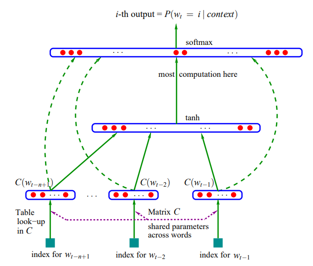
How are these embeddings initialized? They start as random values and are fine-tuned during the backpropagation process. The main purpose of these embeddings is to handle "out-of-distribution" examples, which occur when the language model encounters an input it hasn't seen during training. This can be problematic during inference if the model is fed data that is significantly different from its training data. The embedding approach helps mitigate this by allowing the model to transfer knowledge. For instance, words like "a" and "the" are often interchangeable, so their embeddings will be close in the vector space, enabling the model to generalize. The size of these embeddings is a hyperparameter, which is a key design choice for the neural network.

Building the Dataset

First, let's build the dataset. We'll use a context length of three characters to predict the next one.

# build the dataset
block_size = 3 # context length: how many characters do we take to predict the next one?
X, Y = [], []
for w in words[:5]:
  
  print(w)
  context = [0] * block_size
  for ch in w + '.':
    ix = stoi[ch]
    X.append(context)
    Y.append(ix)
    print(''.join(itos[i] for i in context), '--->', itos[ix])
    context = context[1:] + [ix] # crop and append
  
X = torch.tensor(X)
Y = torch.tensor(Y)

Here are the examples we are feeding our model from the first five names in our dataset:

emma
... ---> e
..e ---> m
.em ---> m
emm ---> a
mma ---> .
olivia
... ---> o
..o ---> l
.ol ---> i
oli ---> v
liv ---> i
ivi ---> a
via ---> .
ava
... ---> a
..a ---> v
.av ---> a
ava ---> .
isabella
... ---> i
..i ---> s
.is ---> a
isa ---> b
sab ---> e
abe ---> l
bel ---> l
ell ---> a
lla ---> .
sophia
... ---> s
..s ---> o
.so ---> p
sop ---> h
oph ---> i
phi ---> a
hia ---> .

The shape and data type of our input X and output Y tensors are:
(torch.Size(), torch.int64, torch.Size(), torch.int64)

Designing the Neural Network

The paper's model used 17,000 words, but our vocabulary only has 27 characters (a-z plus "."). Let's start with 2-dimensional embeddings. Our neural network will take three integers (representing characters) as input and produce one integer as output, just like in the examples above.

There are two ways to conceptualize the embedding layer (matrix C):

1. Indexing into an embedding table to retrieve the vector for an input character.
2. A linear layer with no non-linearity, where the parameters are the matrix C. The code for this would look like: F.one_hot(torch.tensor(5), num_classes=27).float() @ C.

We will stick with the first interpretation, but the second is also a very interesting perspective.

# create the embeddings space
# paper has 17K words, we only have 27 characters
# lets make embedding space 2 dimensional
C = torch.randn((27, 2))

# pytorch indexing is amazing
emb = C[X] 
emb.shape

This gives us a tensor of shape torch.Size(). However, we want a shape of (32, 6) for our hidden layer input. We can use PyTorch's view method to reshape it.

emb.view(32, 6)

Now, let’s initialize the hidden layer. The number of neurons is another hyperparameter; we'll use 100 for now.

W1 = torch.randn((6, 100))
b1 = torch.rand(100)

The output from our hidden layer is calculated as follows:

# pytorch will infer the size for the first element of view()
h = torch.tanh(emb.view(-1, 6) @ W1 + b1) 
h.shape

This results in a tensor of shape torch.Size().

Next, the output layer needs 27 neurons, one for each possible next character.

W2 = torch.randn((100, 27))
b2 = torch.rand(27)
logits = h @ W2 + b2

Recall from our last blog post that we can exponentiate these "logits" to get "fake counts" (since they will all be positive) and then normalize them to get probabilities.

counts = logits.exp() # get fake counts
# Remember broadcasting semantics!
prob = counts / counts.sum(1, keepdims=True) 
prob.shape

The final output of our model before calculating the loss is a tensor of shape torch.Size(). This means for each of our 32 input examples, we have 27 probabilities corresponding to the 27 possible output characters.

Let's find the loss of this untrained network using the negative log-likelihood:

loss = -prob[torch.arange(32), Y].log().mean()
loss

The initial loss is tensor(17.1697). This is quite high, as expected from a forward pass on an untrained, randomly-weighted neural network.

Instead of manually calculating the loss, we can use F.cross_entropy, which combines these steps into a single, efficient function.

loss = F.cross_entropy(logits, Y)

This approach has several advantages:

• It uses fused kernels, which are computationally efficient.
• The backward pass is simpler to compute.
• It is numerically more stable, avoiding issues with large positive numbers during the exp() operation.

Training the Model

Enough talk about the forward pass, let's get to training! First, we build the full dataset.

# build the dataset
block_size = 3 # context length: how many characters do we take to predict the next one?
X, Y = [], []
for w in words:
  context = [0] * block_size
  for ch in w + '.':
    ix = stoi[ch]
    X.append(context)
    Y.append(ix)
    context = context[1:] + [ix] # crop and append
  
X = torch.tensor(X)
Y = torch.tensor(Y)

# Initialize parameters for reproducibility
g = torch.Generator().manual_seed(2147483647) 
C = torch.randn((27, 2), generator=g)
W1 = torch.randn((6, 100), generator=g)
b1 = torch.randn(100, generator=g)
W2 = torch.randn((100, 27), generator=g)
b2 = torch.randn(27, generator=g)
parameters = [C, W1, b1, W2, b2]

# Total number of parameters
sum(p.nelement() for p in parameters) 
# 3481

for p in parameters:
  p.requires_grad = True

Instead of running the forward and backward passes on the entire dataset at once, we'll use mini-batches to make the process more efficient.

for i in range(10000):
  # minibatch construct
  ix = torch.randint(0, X.shape[0], (32, )) # using gradient of 32 random datapoints
  
  # forward pass
  emb = C[X[ix]] # (32, 3, 2)
  h = torch.tanh(emb.view(-1, 6) @ W1 + b1) # (32, 100)
  logits = h @ W2 + b2 # (32, 27)
  loss = F.cross_entropy(logits, Y[ix])

  # backward pass
  for p in parameters:
    p.grad = None # zeros out the grad
  loss.backward()
  
  # update parameters data
  lr = 0.05
  for p in parameters: 
    p.data += -lr * p.grad

The loss at the end of training is 2.1971. This is the loss for the final mini-batch, not the entire training dataset. Using mini-batches is a technique called mini-batch gradient descent, which speeds up training. To get a more accurate view of the model's performance on the whole dataset, we can run a final evaluation:

# how well is the model doing on the whole dataset:
emb = C[X]
h = torch.tanh(emb.view(-1, 6) @ W1 + b1)
logits = h @ W2 + b2
loss = F.cross_entropy(logits, Y)
loss
# 2.5023

Finding the Optimal Learning Rate

How do we determine the best learning rate? We can run a small experiment by testing a range of learning rates and tracking the resulting loss.

lre = torch.linspace(-3, 0, 1000)
lrs = 10 ** lre
lri = []
lossi = []

for i in range(1000):
  # minibatch construct
  ix = torch.randint(0, X.shape[0], (32,))
  
  # forward pass
  emb = C[X[ix]]
  h = torch.tanh(emb.view(-1, 6) @ W1 + b1)
  logits = h @ W2 + b2
  loss = F.cross_entropy(logits, Y[ix])
  
  # backward pass
  for p in parameters:
    p.grad = None
  loss.backward()
  
  # update
  lr = lrs[i]
  for p in parameters:
    p.data += -lr * p.grad
    
  # track stats
  lri.append(lre[i])
  lossi.append(loss.item())

By plotting the loss against the learning rate exponent, we can find a good value.

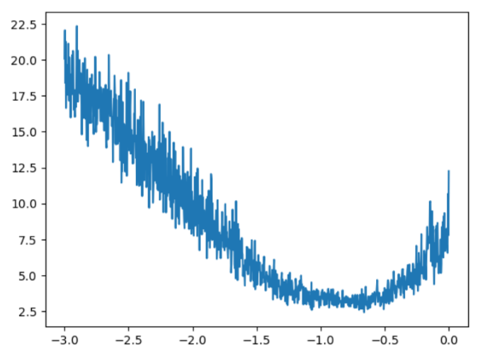
From the plot, we can see that a good learning rate is around 0.1 (which is 10^-1). This simple experiment helps us nail down a good value for this hyperparameter.

Overfitting and Data Splits

Does a lower training loss guarantee a better model? Not necessarily. As a neural network grows larger, it becomes more capable of "overfitting"—memorizing the training data instead of learning to generalize to new, unseen data.

To address this, it's standard practice to split the data into training, validation (or dev), and test sets (typically an 80%, 10%, 10% split).

• Training set: Used to optimize the model's parameters.
• Validation set: Used to tune hyperparameters (like learning rate or embedding size).
• Test set: Used for a final evaluation of the model's performance. This set should be used sparingly to avoid "leaking" information from it into the model design.

Let's apply this to our training loop.

# build the dataset with splits
def build_dataset(words):  
  X, Y = [], []
  for w in words:
    context = [0] * block_size
    for ch in w + '.':
      ix = stoi[ch]
      X.append(context)
      Y.append(ix)
      context = context[1:] + [ix]
  X = torch.tensor(X)
  Y = torch.tensor(Y)
  print(X.shape, Y.shape)
  return X, Y

import random
random.seed(42)
random.shuffle(words)
n1 = int(0.8*len(words))
n2 = int(0.9*len(words))

Xtr, Ytr = build_dataset(words[:n1])
Xdev, Ydev = build_dataset(words[n1:n2])
Xte, Yte = build_dataset(words[n2:])

Here are the sizes for each split:

torch.Size([182625, 3]) torch.Size([182625])
torch.Size([22655, 3]) torch.Size([22655])
torch.Size([22866, 3]) torch.Size([22866])

We re-initialize the parameters and train the model using a learning rate of 0.1. After training for 10,000 iterations, the final mini-batch loss is 2.5190.

Let's check the loss on the full training and validation sets:

Training Loss: tensor(2.3005, grad_fn=)

Validation Loss: tensor(2.3174, grad_fn=)

The training and validation losses are very close, which suggests the model is underfitting. It's not complex enough to capture the patterns in the data. The losses are also higher than what we saw with the bigram model, indicating room for improvement. The embedding dimension and hidden layer size may be bottlenecks.

Scaling Up the Model

Let's increase the model's capacity to see if we can achieve lower losses. We'll increase the embedding dimension from 2 to 10 and the hidden layer size to 200 neurons.

# Change: embedding dim from 2 to 10, hidden layer to 200
g = torch.Generator().manual_seed(2147483647)
C = torch.randn((27, 10), generator=g)
W1 = torch.randn((30, 200), generator=g) # 3 chars * 10 dim = 30
b1 = torch.randn(200, generator=g)
W2 = torch.randn((200, 27), generator=g)
b2 = torch.randn(27, generator=g)
parameters = [C, W1, b1, W2, b2]

sum(p.nelement() for p in parameters)
# 11897 # This is a much bigger model

We'll train this larger model for more iterations, and we can even decay the learning rate partway through training. After training, the loss on the final mini-batch is 2.3348.

Here is the loss plot:

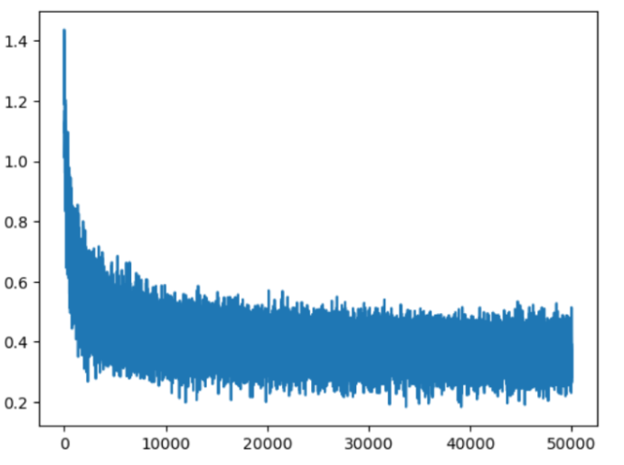
You can see the thickness of the plot towards to right end, indicating the minibatch gives imperfect estimates of the loss.

Let's check the performance on the full sets:

Loss for the entire training set: tensor(2.1647, grad_fn=)

Loss for the validation set: tensor(2.2020, grad_fn=)

These losses are looking a lot better!

Sampling from the Model

Now for the fun part: let's sample from our trained model to see what kind of names it generates.

# sample from the model
g = torch.Generator().manual_seed(2147483647 + 10)

for _ in range(20):
  out = []
  context = [0] * block_size # initialize with all ...
  while True:
    emb = C[torch.tensor([context])] # (1,block_size,d)
    h = torch.tanh(emb.view(1, -1) @ W1 + b1)
    logits = h @ W2 + b2
    probs = F.softmax(logits, dim=1)
    ix = torch.multinomial(probs, num_samples=1, generator=g).item()
    context = context[1:] + [ix]
    out.append(ix)
    if ix == 0:
      break
  
  print(''.join(itos[i] for i in out))

Here are some samples:

carmahfa.
jehleigh.
mili.
tholdence.
saeja.
hubedamerynt.
kaeli.
nellara.
chaiivon.
leggy.
ham.
por.
desian.
sulie.
alian.
quintthoniearyxi.
jacee.
dusabee.
depo.
abetteley.

Compared to the bigram model, these names are much more plausible.

Visualizing Character Embeddings

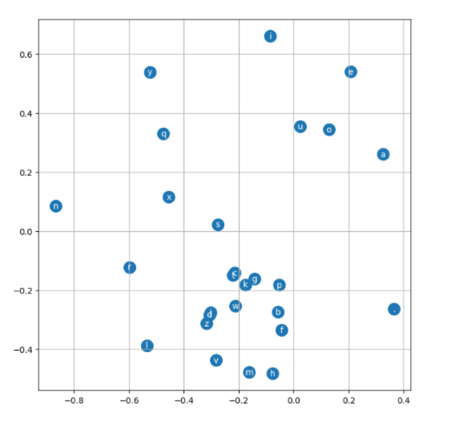
To make the concept of embeddings more concrete, let's visualize the 2D embeddings we trained earlier.

# visualize dimensions 0 and 1 of the embedding matrix C for all characters
plt.figure(figsize=(8,8))
plt.scatter(C[:,0].data, C[:,1].data, s=200)
for i in range(C.shape[0]):
  plt.text(C[i,0].item(), C[i,1].item(), itos[i], ha="center", va="center", color='white')
plt.grid('minor')

During backpropagation, the model learned to position these characters in the embedding space. An interesting finding is that all the vowels are clustered together. This means the model learned to associate vowels with each other. Thanks to this, if the model encounters a vowel in a context it hasn't seen before, it can use what it has learned from other vowels to make a better prediction for the next character.

Here is the plot:

Huge thanks to Andrej Karpathy!