Today we will be reproducing the GPT 2 model, the 124M parameter version. Key references: OpenAI blog post, paper, and code. The 124M parameter model had 12 layers in the transformer and 768 channels in the transformer. The details are somewhat muddy in the GPT 2 paper, so sometimes we will be referencing the GPT 3 paper.
For a sneak peek of the model we build, here is my chatting with the pretrained LLM:
Starting from the End: Pretrained Weights
Let's start from the end. Unlike their newer models, OpenAI actually released the weights for GPT 2. We will download it from Hugging Face because it is PyTorch friendly (the actual OpenAI model is written in TensorFlow). I downloaded GPT 2 (124M parameter version) and inspected the state_dict():
transformer.wte.weight torch.Size([50257, 768])
transformer.wpe.weight torch.Size([1024, 768])
transformer.h.0.ln_1.weight torch.Size([768])
transformer.h.0.ln_1.bias torch.Size([768])
transformer.h.0.attn.c_attn.weight torch.Size([768, 2304])
transformer.h.0.attn.c_attn.bias torch.Size([2304])
transformer.h.0.attn.c_proj.weight torch.Size([768, 768])
transformer.h.0.attn.c_proj.bias torch.Size([768])
transformer.h.0.ln_2.weight torch.Size([768])
transformer.h.0.ln_2.bias torch.Size([768])
transformer.h.0.mlp.c_fc.weight torch.Size([768, 3072])
transformer.h.0.mlp.c_fc.bias torch.Size([3072])
transformer.h.0.mlp.c_proj.weight torch.Size([3072, 768])
transformer.h.0.mlp.c_proj.bias torch.Size([768])
...
transformer.h.11.mlp.c_proj.bias torch.Size([768])
transformer.ln_f.weight torch.Size([768])
transformer.ln_f.bias torch.Size([768])
lm_head.weight torch.Size([50257, 768])
For transformer.wte.weight with shape torch.Size([50257, 768]): there are 50257 tokens in the vocab, exactly the number of tokens we saw in the tokenization lecture. We have a 768 dimensional vector for each token. For transformer.wpe.weight with shape torch.Size([1024, 768]): this is a lookup table for positional embeddings. We have 1024 context for this model and 768 dimensions for each position. The rest is the weights and biases of the network. For example, we can look at the attention weights for some part of our block and visualize it:
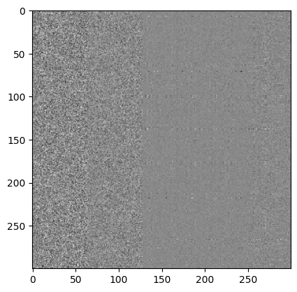
plt.imshow(sd_hf["transformer.h.1.attn.c_attn.weight"][:300,:300], cmap="gray")It would be interesting to try to interpret what this all means, especially for mechanistic interpretability. The definition of mechanistic interpretability: "Mechanistic interpretability seeks to reverse engineer neural networks, similar to how one might reverse engineer a compiled binary computer program" (Anthropic). Not only do we have the weights, but we can actually load the pipeline and sample from the model!
from transformers import pipeline, set_seed
generator = pipeline('text-generation', model='gpt2')
set_seed(42)
generator("Hello, I'm a language model,", max_length=30, num_return_sequences=1)
Example output:
[{'generated_text': 'Hello, I\'m a language model, so you can\'t just use the same data model...'}]We can load the model, we can look at the parameters, the keys tell us where we are in the model. We want to write our own GPT class so we have full understanding. Understanding transformers' implementation is going to be difficult because of how dense the code is. First lets try to load the pretrained model into our class, then we will initialize the weights from scratch from our own documents.
Architecture: GPT-2 vs. Attention is All You Need
Let's go to the Attention is All You Need paper. Remember the GPT 2 transformer is not the same as the transformer proposed there. That one was an encoder-decoder model. GPT 2 is decoder only. Cross attention that was using the encoder is also missing in GPT 2. Other differences in GPT 2: first, reshuffling the layer norms so that layer norms happen before MLP or attention rather than at the end. Second, they added a layer norm at the end of the decoder blocks.
GPT Skeleton
Alright so let's try to create a skeleton of GPT 2 in VS Code, matching what we saw here. Loading the weights gives us the same structure. Here is what we came up with to match this:
class GPT(nn.Module):
    def __init__(self, config):
        super().__init__()
        self.config = config

        self.transformer = nn.ModuleDict(dict(
            wte = nn.Embedding(config.vocab_size, config.n_embd),
            wpe = nn.Embedding(config.block_size, config.n_embd),
            h = nn.ModuleList([Block(config) for _ in range(config.n_layer)]),
            ln_f = nn.LayerNorm(config.n_embd),
        ))
        self.lm_head = nn.Linear(config.n_embd, config.vocab_size, bias=False)

# Block class to be implemented

class Block(nn.Module):
    def __init__(self, config):
        super().__init__()
        self.ln_1 = nn.LayerNorm(config.n_embd)
        self.attn = CausalSelfAttention(config)
        self.ln_2 = nn.LayerNorm(config.n_embd)
        self.mlp = MLP(config)

    def forward(self, x):
        x = x + self.attn(self.ln_1(x))
        x = x + self.mlp(self.ln_2(x))
        return x
You can see from above that the layer normalizations are before the MLP and attention heads. Additionally in the Attention is All You Need transformer, the layer norms are "in the residual pathway." This is undesirable, and GPT 2 changed this so that the layer norms are on the branch to MLP and self-attention (and our above code reflects this as well). Why is this desirable? Well as mentioned when we were building our small GPT in the previous blog post, as much as possible we want our residual path to be clean. The whole point of the residual pathway is so that when we do backpropagation, we send the gradients back to the input. As we start training, the gradients start off by impacting the inputs first, but as training continues the branches of MLP and attention start becoming online increasingly.
Remember attention is a communication mechanism where tokens exchange their information. It is a reduce operation, it is a weighted sum operation. The MLP (aka Feed forward network) is an operation that works on each token individually. This is where each token "thinks" about the information it has gathered. It is a Map operation. So what happens is in one attention block we do a Map Reduce, repeatedly. Another way to think about this: attention is a sequence mixer, allowing different tokens to communicate amongst each other. MLP is a channel mixer: the channels of a single token get time to think together.
MLP Module
How do we implement the MLP module?
class MLP(nn.Module):
    def __init__(self, config):
        super().__init__()
        self.c_fc    = nn.Linear(config.n_embd, 4 * config.n_embd)
        self.gelu    = nn.GELU(approximate='tanh')
        self.c_proj  = nn.Linear(4 * config.n_embd, config.n_embd)

    def forward(self, x):
        x = self.c_fc(x)
        x = self.gelu(x)
        x = self.c_proj(x)
        return x
This is relatively straightforward. You have the GELU nonlinearity sandwiched between two projection layers. You might notice that we are using the approximate hyperparameter. Why are we doing this? According to Andrej Karpathy, there is no real good reason for using this right now. It is more of a historical quirk. We are using it here because GPT 2 used it, and we want to be as exact as possible. Another reason to use GELU is the dead neuron problem with ReLU. Activations that fall in the flat tail of ReLU will get exactly 0 gradient. That means that the neuron will stop learning because it is essentially dead. GELU slightly fixes this by smoothing this tail so that it is not exactly 0, and therefore the neuron is still learning even if it is on the flat tail. Note the c_proj at the very end of the forward(). We do this projection to make sure right before we return back to the residual stream (the gradient super highway we talked about earlier). This pattern happens in the attention operation below as well.
Causal Self-Attention
Now let's go to the attention operation:
class CausalSelfAttention(nn.Module):
    def __init__(self, config):
        super().__init__()
        assert config.n_embd % config.n_head == 0
        # key, query, value projections for all heads, but in a batch
        self.c_attn = nn.Linear(config.n_embd, 3 * config.n_embd)
        # output projection
        self.c_proj = nn.Linear(config.n_embd, config.n_embd)
        # regularization
        self.n_head = config.n_head
        self.n_embd = config.n_embd
        # not really a 'bias', more of a mask, but following the OpenAI/HF naming
        self.register_buffer("bias", torch.tril(torch.ones(config.block_size, config.block_size))
                                     .view(1, 1, config.block_size, config.block_size))

    def forward(self, x):
        B, T, C = x.size()  # batch size, sequence length, embedding dimensionality (n_embd)
        # calculate query, key, values for all heads in batch and move head forward to be the batch dim
        # nh is "number of heads", hs is "head size", and C (number of channels) = nh * hs
        # e.g. in GPT-2 (124M), n_head=12, hs=64, so nh*hs=C=768 channels in the Transformer
        qkv = self.c_attn(x)
        q, k, v = qkv.split(self.n_embd, dim=2)
        k = k.view(B, T, self.n_head, C // self.n_head).transpose(1, 2)  # (B, nh, T, hs)
        q = q.view(B, T, self.n_head, C // self.n_head).transpose(1, 2)  # (B, nh, T, hs)
        v = v.view(B, T, self.n_head, C // self.n_head).transpose(1, 2)  # (B, nh, T, hs)
        # attention (materializes the large (T,T) matrix for all the queries and keys)
        att = (q @ k.transpose(-2, -1)) * (1.0 / math.sqrt(k.size(-1)))
        att = att.masked_fill(self.bias[:,:,:T,:T] == 0, float('-inf'))
        att = F.softmax(att, dim=-1)
        y = att @ v  # (B, nh, T, T) x (B, nh, T, hs) -> (B, nh, T, hs)
        y = y.transpose(1, 2).contiguous().view(B, T, C)  # re-assemble all head outputs side by side
        # output projection
        y = self.c_proj(y)
        return y
This specifically implements multi headed self attention. Last time in our implementation we had a separate multi headed attention module and a single head of attention module. The difference being that multi headed attention is simply multiple heads of attention running in parallel and their results being concatenated at the end. Now we combine these two modules to put it in a single self attention module so that the multi heads are just an extra batch dimension.
Here is a recap of how the attention operation works here: We get an input sequence of shape B T C (B is batch size, T is time dimension or the sequence length, and C is the embeddings dimensionality / n_embd). We pass the input into c_attn to get a tensor of shape B T 3C. We split this amongst the 2nd dimension to get our q k v each of size B T n_embd. Essentially we have converted our input of shape B T C into B T n_embd by getting the queries keys and values associated with each token independently. This conversion happens in c_attn. We do some tensor gymnastics to get shape B nh T hs (where nh is number of heads and hs is the head size). We essentially just split the n_embd into nh and hs (nh * hs = n_embd). We did this so that we can treat the nh (number of heads) dimension as a batch dimension because we are treating each head independently in parallel. To get our affinities matrix (to use terminology from our last blog post) we multiply queries matrix with our keys matrix, and divide by the square root of the keys head size following the Attention is All You Need paper. If we think about the shapes this will be B nh T hs @ B nh T hs to B nh T T. This shape should look familiar based off of our last blog posts: for each batch, for each head, we now have a T by T affinities matrix telling us how similar each token is based off of their queries representing "what am I looking for?" and the key vector representing "what do I contain?" We do the masked fill on this B nh T T to make sure tokens can't look at their future tokens, and softmax across the "rows" (the last T dimension) to make sure the sum of the exponents is 1 row wise. When we do y = att @ v, the shapes here are: B nh T T @ B nh T hs to B nh T hs. Remember if the queries are asking "what am I looking for", and keys are representing "what do I contain", the values contain "if you find me interesting, here is what I will communicate to you." The next line of code transposes the 1st and 2nd dimension (0 indexed) to get the shape B T nh hs, and then combines the last two dimensions to get a B T C tensor. We have essentially concatenated each head's output. We will run through this projection to get the same shape, a B T C tensor. We are done with communicating across tokens using the attention operation!
Andrej was very careful about his naming convention here. We need to match the names of each tensor if we hope to port all the weights into our custom class. At this point we are able to pull the weights released from GPT 2, set them, and do some generation. We also had to change the following to match the GPT 2 hyperparameters:
@dataclass
class GPTConfig:
    block_size: int = 1024  # max sequence length
    vocab_size: int = 50257  # number of tokens: 50,000 BPE merges + 256 bytes tokens + 1 <|endoftext|> token
    n_layer: int = 12  # number of layers
    n_head: int = 12  # number of heads
    n_embd: int = 768  # embedding dimension
Now to port the weights we have to use the following code:
@classmethod
def from_pretrained(cls, model_type):
    """Loads pretrained GPT-2 model weights from huggingface"""
    assert model_type in {'gpt2', 'gpt2-medium', 'gpt2-large', 'gpt2-xl'}
    from transformers import GPT2LMHeadModel
    print("loading weights from pretrained gpt: %s" % model_type)

    # n_layer, n_head and n_embd are determined from model_type
    config_args = {
        'gpt2':         dict(n_layer=12, n_head=12, n_embd=768),   # 124M params
        'gpt2-medium':  dict(n_layer=24, n_head=16, n_embd=1024),  # 350M params
        'gpt2-large':   dict(n_layer=36, n_head=20, n_embd=1280),  # 774M params
        'gpt2-xl':      dict(n_layer=48, n_head=25, n_embd=1600),  # 1558M params
    }[model_type]
    config_args['vocab_size'] = 50257  # always 50257 for GPT model checkpoints
    config_args['block_size'] = 1024   # always 1024 for GPT model checkpoints
    # create a from-scratch initialized minGPT model
    config = GPTConfig(**config_args)
    model = GPT(config)
    sd = model.state_dict()
    sd_keys = sd.keys()
    sd_keys = [k for k in sd_keys if not k.endswith('.attn.bias')]  # discard this mask / buffer, not a param

    # init a huggingface/transformers model
    model_hf = GPT2LMHeadModel.from_pretrained(model_type)
    sd_hf = model_hf.state_dict()

    # copy while ensuring all of the parameters are aligned and match in names and shapes
    sd_keys_hf = sd_hf.keys()
    sd_keys_hf = [k for k in sd_keys_hf if not k.endswith('.attn.masked_bias')]  # ignore these, just a buffer
    sd_keys_hf = [k for k in sd_keys_hf if not k.endswith('.attn.bias')]  # same, just the mask (buffer)
    transposed = ['attn.c_attn.weight', 'attn.c_proj.weight', 'mlp.c_fc.weight', 'mlp.c_proj.weight']
    # basically the openai checkpoints use a "Conv1D" module, but we only want to use a vanilla Linear
    # this means that we have to transpose these weights when we import them
    assert len(sd_keys_hf) == len(sd_keys), f"mismatched keys: {len(sd_keys_hf)} != {len(sd_keys)}"
    for k in sd_keys_hf:
        if any(k.endswith(w) for w in transposed):
            # special treatment for the Conv1D weights we need to transpose
            assert sd_hf[k].shape[::-1] == sd[k].shape
            with torch.no_grad():
                sd[k].copy_(sd_hf[k].t())
        else:
            # vanilla copy over the other parameters
            assert sd_hf[k].shape == sd[k].shape
            with torch.no_grad():
                sd[k].copy_(sd_hf[k])

    return model
So the from_pretrained() is a classmethod that returns the GPT object given the model name. When we run it we see:
(venv) oagrawal@mew3:/nfs/oagrawal/andrej/build-nanogpt$ python3 train_gpt2.py
loading weights from pretrained gpt: gpt2
Loading weights: 100%|█████████████████████████| 148/148 [00:00<00:00, 3620.65it/s, Materializing param=transformer.wte.weight]
Now how do we sample from this model?
def forward(self, idx):
    # idx is of shape (B, T)
    B, T = idx.size()
    assert T <= self.config.block_size, f"Cannot forward sequence of length {T}, block size is only {self.config.block_size}"
    # forward the token and position embeddings
    pos = torch.arange(0, T, dtype=torch.long, device=idx.device)  # shape (T)
    pos_emb = self.transformer.wpe(pos)   # position embeddings of shape (T, n_embd)
    tok_emb = self.transformer.wte(idx)   # token embeddings of shape (B, T, n_embd)
    x = tok_emb + pos_emb
    # forward the blocks of the transformer
    for block in self.transformer.h:
        x = block(x)
    # forward the final layernorm and the classifier
    x = self.transformer.ln_f(x)
    logits = self.lm_head(x)  # (B, T, vocab_size)
    return logits
Forward pass details: The input is shape B T. To get the token_embeddings, we will pass this B T tensor into self.transformer.wte to get the embedding for each token independently (the shape of this tensor will now be B T n_embd). To get the position embeddings we first create a single dimension torch tensor that has elements 0 to T-1 (it will look like [0 1 2 ... T-1]). We pass it through self.transformer.wpe to get the position embedding for each token which will be of shape T n_embd. We will add these two tensors to get x (shape B T n_embd). How does this addition work if these two inputs are of different sizes? There is a hidden broadcast operation here, where B T n_embd + T n_embd: the second tensor will get right aligned and get another dimension added to the beginning that matches the first B dimension. This will give us B T n_embd + B T n_embd. This addition is simply element wise addition now. Now we pass these inputs through the decoder blocks, which maintain their shape (B T n_embd). We pass the last x into self.transformer.ln_f, and this layer norm maintains the shape. Finally we pass this input into self.lm_head, which changes the input shape from B T n_embd to B T vocab_size. These are the logits, and are one step from getting the probabilities of the next token to sample the next token.
Now here is how we will call this forward block:
num_return_sequences = 5
max_length = 30

model = GPT.from_pretrained('gpt2')
model.eval()
model.to('cuda')
Here we are replicating the earlier example we had for our jupyter notebook (with 5 parallel generations of max length 30 tokens). We set the model to eval() mode. This actually doesn't do anything in terms of the modules we programmed (because at training and test time all of our modules run identically; if we had a dropout or batch norm layer somewhere the story would be different). We are setting this model to eval mode partly for good practice's sake. Partly because there might be some clever optimization PyTorch does under the hood. Then we transfer the model to cuda. Essentially the way to think about this is the model is on our machine, so when we transfer the model to cuda we are transferring to the GPU. While the GPU is another device connected to our computer, this GPU has a completely different architecture than our current machine which allows it to do parallel computations extremely efficiently.
# prefix tokens
import tiktoken
enc = tiktoken.get_encoding('gpt2')
tokens = enc.encode("Hello, I'm a language model,")
tokens = torch.tensor(tokens, dtype=torch.long)  # (8,)
tokens = tokens.unsqueeze(0).repeat(num_return_sequences, 1)  # (5, 8)
x = tokens.to('cuda')
When we do tokens = enc.encode("Hello, I'm a language model,") we are getting a list of numbers that identify "Hello, I'm a language model". We then encode this list into a tensor, and then when we run tokens = tokens.unsqueeze(0).repeat(num_return_sequences, 1) we are replicating these numbers 5 times on the 0th dimension. The resulting tensor is a 5 by 8 tensor, where the 5 rows have the same values. Here too we will transfer this memory to the GPU by doing tokens.to('cuda'). We can now pass x into the forward function to get the logits to get the model's prediction for the next token. See code below:
# generate! right now x is (B, T) where B = 5, T = 8
# set the seed to 42
torch.manual_seed(42)
torch.cuda.manual_seed(42)
while x.size(1) < max_length:
    # forward the model to get the logits
    with torch.no_grad():
        logits = model(x)  # (B, T, vocab_size)
        # take the logits at the last position
        logits = logits[:, -1, :]  # (B, vocab_size)
        # get the probabilities
        probs = F.softmax(logits, dim=-1)
        # do top-k sampling of 50 (huggingface pipeline default)
        # topk_probs here becomes (5, 50), topk_indices is (5, 50)
        topk_probs, topk_indices = torch.topk(probs, 50, dim=-1)
        # select a token from the top-k probabilities
        # note: multinomial does not demand the input to sum to 1
        ix = torch.multinomial(topk_probs, 1)  # (B, 1)
        # gather the corresponding indices
        xcol = torch.gather(topk_indices, -1, ix)  # (B, 1)
        # append to the sequence
        x = torch.cat((x, xcol), dim=1)
Sampling loop: We start with a 5 by 8 tensor, but for each iteration (until max_length columns) we are sampling from the model. We can make a prediction for the next character for each batch request, and we append this predicted token to the end of this tensor. So we are transforming the x tensor shape from 5 by 8 to 5 by 9 to 5 by 10, etc. In other words for each iteration we are adding a new column. Note that the with torch.no_grad() tells PyTorch that it doesn't have to store the gradient for these values. Remember that regularly when we do any operation with objects in PyTorch, it keeps track of the current value, the gradient of the value, and the underlying computational graph of how objects are related to each other. This makes backpropagation extremely easy, but because here we are just writing code for inference, we will never call loss.backward() on this, so this context manager tells PyTorch that it doesn't need to do all that extra work. This will save us space. Let's go through the shapes here too: We pass x into the model.forward(). X has shape B T, to get logits of size B T vocab_size. We only care about the predictions for the last token, so our logits are now B vocab_size. We apply a softmax on the last dimension to get the probabilities for each batch element's next character. Now here is something interesting: respecting the way Hugging Face pipeline does it, we take the top 50 most likely tokens for each batch, and set the rest of the tokens to 0. This way we stabilize inference in a way, and we are not deviating too much from the predicted next characters. At this point the input is a B 50 tensor. We sample a token from these top 50 likely tokens to get a tensor of B by 1 (this is the multinomial and gather steps). And at the end we append this new column of indices to x, and repeat this until the size of x hits the max_length (which in this case we had set max_length being 30). To make this human translatable, for each tokens for each batch we call the enc.decode() function:
# print the generated text
for i in range(num_return_sequences):
    tokens = x[i, :max_length].tolist()
    decoded = enc.decode(tokens)
    print(">", decoded)
Example output when running with pretrained weights:
> Hello, I'm a language model, not a program.
So this morning I started studying for the interview in the lab. This was not
> Hello, I'm a language model, and one of the main things that bothers me when they create languages is how easy it becomes to create something that
> Hello, I'm a language model, and I wrote it off on the grounds that a language model would make me more fluent. But I'm not
> Hello, I'm a language model, I really like languages. I like languages because like, they're good. And the way we talk about languages
> Hello, I'm a language model, a language model I'm using for data modelling. All I did was test the results and then I wrote some
Andrej Karpathy did this manually with the Hugging Face version of the model, and got the same 5 outputs. This way we know that the model internals are correct. So now we have GPT 2 model, the exact same model OpenAI developed several years ago. That is awesome. We can now poke around and explore this model a bit more. What we want to do now is reinitialize the weights and train this model from scratch, so that we can get these weights on our own, and potentially even exceed the performance of this model OpenAI trained. Turns out getting the random model isn't that hard:
# model = GPT.from_pretrained('gpt2')
model = GPT(GPTConfig())
Instead of calling from_pretrained() to get the model weights that OpenAI had, by default PyTorch initializes all of these weights to be random, and all we need to pass in is the GPTConfig where we define the major hyperparameters of the network. If we run inference again we see that we get totally random outputs:
(venv) oagrawal@mew3:/nfs/oagrawal/andrej/build-nanogpt$ python3 train_gpt2.py
using device: cuda
> Hello, I'm a language model, pictured uncontrolled Downs rocky ladderrehensive Cla ecc alright'). Almost Rose444 RFCictions guidelines exposures dealers Druid adaptation882ythm
> Hello, I'm a language model,ople organisations quickeal PIT symbolic Vu II contextilar headsets struct versatility Merchant heroic canceledpublichyp bunk ed filename Kerr
> Hello, I'm a language model, bound196foundedifies noting demeanor leng patriarch circumcised refresARP 1944Incre developmental BP officers modes battledarf mars Spring maj
> Hello, I'm a language model, accepts Sheila Kus Sheila sir Numerous wonderful outbreak approves Carry recovered Stainaturally kits Damikuman MVP sorcerer"}],"117 accumulate Liu
> Hello, I'm a language model,aura generalsigenilde chocolate extermination Gothaucletters Brewerszanrichfixes Radio formulations noon standby likedviolentDutch strategy power
(venv) oagrawal@mew3:/nfs/oagrawal/andrej/build-nanogpt$
Andrej also likes to autodetect the device that has the highest compute capability:
device = "cpu"
if torch.cuda.is_available():
    device = "cuda"
elif hasattr(torch.backends, "mps") and torch.backends.mps.is_available():
    device = "mps"
print(f"using device: {device}")
Now with this variable "device", instead of sending buffers to cuda, we can send to device by doing .to(device).
Training the Model
Let's get to training the model. Let's get a dataset. Similar to the previous blog post let's get the Tiny Shakespeare dataset. Let's read in the first 1000 characters of this dataset to see what it looks like:
# tiny shakespeare dataset
# !wget https://raw.githubusercontent.com/karpathy/char-rnn/master/data/tinyshakespeare/input.txt
with open('input.txt', 'r') as f:
    text = f.read()
data = text[:1000]  # first 1,000 characters
print(data[:100])
Output:
First Citizen:
Before we proceed any further, hear me speak.

All:
Speak, speak.

First Citizen:
You
Now let's use the GPT2 tokenizer to encode the dataset into a sequence of tokens:
import tiktoken
enc = tiktoken.get_encoding('gpt2')
tokens = enc.encode(data)
print(tokens[:24])
Output: [5962, 22307, 25, 198, 8421, 356, 5120, 597, 2252, 11, 3285, 502, 2740, 13, 198, 198, 3237, 25, 198, 5248, 461, 11, 2740, 13]
Now, if you remember our model expects a model input of shape B x T, not a long single input. In our jupyter notebook, let's say T is 6 and B is 4. We can get the first 24 tokens and .view() this tensor to arrange this tensor according to the forward() function's input. We have the input. What about the expected output? Our model training is supervised, so we need to have the "correct answer" (e.g. correct next token) for each token for each batch of the input. To get the correct output, we will read in the first 25 tokens (one additional token), and reshape the 24 tokens starting from the 2nd token (we will skip the first token). Here is that in code:
import torch
buf = torch.tensor(tokens[:24 + 1])
x = buf[:-1].view(4, 6)
y = buf[1:].view(4, 6)
print(x)
print(y)
Output:
tensor([[ 5962, 22307,    25,   198,  8421,   356],
        [ 5120,   597,  2252,    11,  3285,   502],
        [ 2740,    13,   198,   198,  3237,    25],
        [  198,  5248,   461,    11,  2740,    13]])
tensor([[22307,    25,   198,  8421,   356,  5120],
        [  597,  2252,    11,  3285,   502,  2740],
        [   13,   198,   198,  3237,    25,   198],
        [ 5248,   461,    11,  2740,    13,   198]])
Let's try to run a small test input into our model, and see what the output looks like:
# get a data batch
import tiktoken
enc = tiktoken.get_encoding('gpt2')
with open('input.txt', 'r') as f:
    text = f.read()
text = text[:1000]
tokens = enc.encode(text)
B, T = 4, 32
buf = torch.tensor(tokens[:B*T + 1])
x = buf[:-1].view(B, T)
y = buf[1:].view(B, T)

# get logits
model = GPT(GPTConfig())
model.to(device)
logits = model(x)
print(logits.shape)
Output:
(venv) oagrawal@mew3:/nfs/oagrawal/andrej/build-nanogpt$ python3 train_gpt2.py
using device: cuda
torch.Size([4, 32, 50257])
For each batch for each token, there is a 50257 dimension vector for the prediction of the next token (there are 50257 possible next tokens). Now let's calculate the loss and do the backward pass and do the optimization. We will need to adjust the forward function: we will pass in input indices and targets, we won't just pass logits but also the loss. We will be using the cross entropy loss:
loss = F.cross_entropy(logits.view(-1, logits.size(-1)), targets.view(-1))What is going on here is logits is going from a B by T by C tensor to a B*T by C vector. The target is going from B by T to a B*T single dimensional tensor. Cross entropy turns the logits for each token into a probability distribution for the next token. Then we use the probability for the correct next token for the loss. Let's see what the initial loss for our uninitialized model is:
model = GPT(GPTConfig())
model.to(device)
logits, loss = model(x, y)
print(loss)
import sys; sys.exit(0)
Output:
(venv) oagrawal@mew3:/nfs/oagrawal/andrej/build-nanogpt$ python3 train_gpt2.py
using device: cuda
tensor(11.0699, grad_fn=<NllLossBackward0>)
How can we make sure this number makes sense? For this let's make sure we understand how F.cross_entropy works under the hood. Remember that cross entropy is the negative log likelihood we saw in previous lectures. Likelihood is the product of the probabilities assigned to the correct next character for all bigrams in the dataset. We are feeding in logits to the cross entropy function for each token, so we will use softmax to convert these logits to probabilities for each token. Then using the target, we will extract the model output's probability for the correct next token. Using these probabilities we will multiply all of these probabilities to get the "likelihood". Since these probabilities are all between 0 and 1, the likelihood will be a very small number for all n numbers, so we will take the log of this likelihood. Because the likelihood was between 0 and 1, the log of this number will be negative. Currently when the likelihood is better (closer to 1) we have a less negative number, but a characteristic we want our loss function to have is lower number should be better. So we take the negative of this log likelihood. And finally, we will average this across all training examples (n). Back to sanity checking the loss value we got: it would make sense at initialization for all probabilities to be pretty equal. So because we have 50257 tokens, we want our correct next token (at initialization at least) to be 1/50257. The likelihood would be 1/50257 ** n. So the negative log likelihood is -ln(1/50257 ** n), and the average NLL would be -ln(1/50257 ** n) / n = -ln(1/50257) = 10.82. 11.06 and 10.82 is pretty similar, which tells us that our probability distributions are fairly diffused and we expect to get a loss value similar to 11.06.
Let's get started with the optimization. Let's create the Adam optimizer object. Remember from an earlier blog post that the optimizer essentially updates the parameter with the gradient times the learning rate (it is the algorithm used to update weights to minimize the loss function). In addition to this Adam keeps two buffers around: the m (first moment) and v (second moment). It is kind of like a normalization for each gradient element individually, faster than SGD.
optimizer = torch.optim.AdamW(model.parameters(), lr=3e-4)
for i in range(50):
    optimizer.zero_grad()
    logits, loss = model(x, y)
    loss.backward()
    optimizer.step()
    print(f"step {i}, loss: {loss.item()}")
Now let's see what our losses look like for the small test input we had above:
(venv) oagrawal@mew2:/nfs/oagrawal/andrej/build-nanogpt$ python3 train_gpt2.py
using device: cuda
step 0, loss: 10.982768058776855
step 1, loss: 6.584049224853516
step 2, loss: 4.2438154220581055
step 3, loss: 2.592557907104492
step 4, loss: 1.5058900117874146
step 5, loss: 0.8241760730743408
step 6, loss: 0.47475460171699524
step 7, loss: 0.27522769570350647
step 8, loss: 0.1787755787372589
step 9, loss: 0.11873787641525269
step 10, loss: 0.07977631688117981
step 11, loss: 0.059421196579933167
step 12, loss: 0.047055166214704514
step 13, loss: 0.0374368280172348
step 14, loss: 0.03118971735239029
step 15, loss: 0.027477802708745003
step 16, loss: 0.024734828621149063
step 17, loss: 0.022128723561763763
step 18, loss: 0.01949634589254856
step 19, loss: 0.016981080174446106
step 20, loss: 0.014903114177286625
step 21, loss: 0.013259010389439212
step 22, loss: 0.011918843723833561
step 23, loss: 0.010789178311824799
step 24, loss: 0.009823054075241089
step 25, loss: 0.008994294330477715
step 26, loss: 0.008280778303742409
step 27, loss: 0.0076614003628492355
step 28, loss: 0.007119027432054281
step 29, loss: 0.006641101557761431
step 30, loss: 0.006218414753675461
step 31, loss: 0.005843899678438902
step 32, loss: 0.005511464551091194
step 33, loss: 0.005215596407651901
step 34, loss: 0.004951337352395058
step 35, loss: 0.0047143250703811646
step 36, loss: 0.004500805400311947
step 37, loss: 0.004307546652853489
step 38, loss: 0.004131893627345562
step 39, loss: 0.00397167494520545
step 40, loss: 0.0038251017685979605
step 41, loss: 0.0036905985325574875
step 42, loss: 0.003566993400454521
step 43, loss: 0.0034531184937804937
step 44, loss: 0.003348063211888075
step 45, loss: 0.003250989131629467
step 46, loss: 0.003161204978823662
step 47, loss: 0.003078003413975239
step 48, loss: 0.003000872442498803
step 49, loss: 0.0029291408136487007
(venv) oagrawal@mew2:/nfs/oagrawal/andrej/build-nanogpt$
The .zero_grad() is important. Later when we get the losses and do loss.backward(), loss.backward() does a += operation, so that is why we need to zero the gradient with .zero_grad() at the beginning of the optimization loop. loss.backward() finds the gradient of the loss with respect to each parameter in our network. Remember in PyTorch each object has a value and its gradient. This step fills in the gradient value. We need to do optimizer.step() to actually update the value according to gradient for each parameter in our network.
When training on the same small test input for 50 steps, we see losses drop very quickly (from ~11 to ~0.003). We see that we are getting pretty low losses! Now we need to change the optimization so that instead of training on the same subset of the data 50 times, we train on a different subset of the data 50 times. That way we are optimizing for a reasonable objective, which is "learning" the entire dataset rather than just memorizing the first couple tokens. For this, we will create an object called a dataloader:
# -----------------------------------------------------------------------------
import tiktoken

class DataLoaderLite:
    def __init__(self, B, T):
        self.B = B
        self.T = T

        # at init load tokens from disk and store them in memory
        with open('input.txt', 'r') as f:
            text = f.read()
        enc = tiktoken.get_encoding('gpt2')
        tokens = enc.encode(text)
        self.tokens = torch.tensor(tokens)
        print(f"loaded {len(self.tokens)} tokens")
        print(f"1 epoch = {len(self.tokens) // (B * T)} batches")

        # state
        self.current_position = 0

    def next_batch(self):
        B, T = self.B, self.T
        buf = self.tokens[self.current_position : self.current_position+B*T+1]
        x = (buf[:-1]).view(B, T)  # inputs
        y = (buf[1:]).view(B, T)   # targets
        # advance the position in the tensor
        self.current_position += B * T
        # if loading the next batch would be out of bounds, reset
        if self.current_position + (B * T + 1) > len(self.tokens):
            self.current_position = 0
        return x, y

# -----------------------------------------------------------------------------
Essentially what happens here is we specify the batch and time dimension we want our model to have for each generation. We then load the entire dataset and walk the dataset in steps of size B*T at a time. Once we get to the end of the entire dataset, we call that one epoch. Measuring in epochs is important because it measures how many complete passes the model has seen. This is our updated optimization loop:
train_loader = DataLoaderLite(B=4, T=32)

# get logits
model = GPT(GPTConfig())
model.to(device)

# optimize!
optimizer = torch.optim.AdamW(model.parameters(), lr=3e-4)
for i in range(50):
    x, y = train_loader.next_batch()
    x, y = x.to(device), y.to(device)
    optimizer.zero_grad()
    logits, loss = model(x, y)
    loss.backward()
    optimizer.step()
    print(f"step {i}, loss: {loss.item()}")
Here are the losses now:
(venv) oagrawal@mew3:/nfs/oagrawal/andrej/build-nanogpt$ python3 train_gpt2.py
using device: cuda
loaded 338025 tokens
1 epoch = 2640 batches
step 0, loss: 10.978148460388184
step 1, loss: 9.684946060180664
step 2, loss: 8.639444351196289
step 3, loss: 8.961030960083008
step 4, loss: 8.441011428833008
step 5, loss: 8.1319580078125
step 6, loss: 8.922016143798828
step 7, loss: 8.665694236755371
step 8, loss: 8.081135749816895
step 9, loss: 7.851987838745117
step 10, loss: 8.198379516601562
step 11, loss: 7.135965347290039
step 12, loss: 7.6971635818481445
step 13, loss: 7.214962005615234
step 14, loss: 7.4223151206970215
step 15, loss: 7.105324745178223
step 16, loss: 7.301327705383301
step 17, loss: 8.268877029418945
step 18, loss: 7.052347183227539
step 19, loss: 7.67573356628418
step 20, loss: 7.41237735748291
step 21, loss: 7.569397926330566
step 22, loss: 6.1853532791137695
step 23, loss: 6.597555637359619
step 24, loss: 6.583559036254883
step 25, loss: 6.222142219543457
step 26, loss: 6.398843765258789
step 27, loss: 7.473003387451172
step 28, loss: 6.935136318206787
step 29, loss: 6.6142802238464355
step 30, loss: 6.918460845947266
step 31, loss: 6.915646553039551
step 32, loss: 6.877722263336182
step 33, loss: 6.621794700622559
step 34, loss: 7.874507904052734
step 35, loss: 7.71798849105835
step 36, loss: 7.386514663696289
step 37, loss: 7.449836730957031
step 38, loss: 7.479292869567871
step 39, loss: 7.153037071228027
step 40, loss: 7.217015743255615
step 41, loss: 6.265650749206543
step 42, loss: 6.623948097229004
step 43, loss: 6.712372303009033
step 44, loss: 6.613269805908203
step 45, loss: 6.574107646942139
step 46, loss: 5.658519268035889
step 47, loss: 5.989255905151367
step 48, loss: 6.81461763381958
step 49, loss: 6.502427101135254
(venv) oagrawal@mew3:/nfs/oagrawal/andrej/build-nanogpt$
With the dataloader, the losses go down but at a much lower rate. This is because previously we were just overfitting one batch but now we are using different batches, so the learning will be slower. Andrej thinks these gains are along the lines of eliminating usage of certain tokens (Tiny Shakespeare is only using a very small subset of the 50257 tokens we have in our vocabulary). There are some very easy gains to be made with this, for example setting the weights such that the tokens that never occur in the dataset have an extremely low probability of being outputted as the next token. The model is probably trying to delete the use of the tokens that it's never seen yet.
Parameter Sharing
Parameter sharing between token embedding and the output lm_head: currently our model isn't exactly structured as the GPT 2 model was. Specifically, in GPT 2, OpenAI used the same tensor they used in the wte tensor (token embeddings matrix) and the lm_head (the linear layer used after the attention block and the final layer norm, to convert the input from B T n_embd to B T vocab_size, to get to the next token). Why do they do this? Well they cite the following paper (Using the Output Embedding to Improve Language Models: https://arxiv.org/pdf/1608.05859), where they discover that the output linear layer acts very similar to an embeddings matrix, and that if you actually make both of these components the same the model performance improves. We currently have two different tensors for this, so we need to change our model to follow OpenAI's implementation! Another benefit: this matrix believe it or not has a large portion of the model's parameters! These matrices have 768 * 50257 which is approximately 40,000,000 parameters. This is like 30% of the 124M parameters. By sharing these parameters you don't have to train as many parameters, and you become more efficient in terms of the training process.
We implement the parameter sharing pretty simply in the GPT class by doing the following:
self.transformer.wte.weight = self.lm_head.weightWeight Initialization
Okay we have a simple optimization loop. Now let's try to make our initialization of weights a little smarter:
def _init_weights(self, module):
    if isinstance(module, nn.Linear):
        std = 0.02
        if hasattr(module, 'NANOGPT_SCALE_INIT'):
            std *= (2 * self.config.n_layer) ** -0.5
        torch.nn.init.normal_(module.weight, mean=0.0, std=std)
        if module.bias is not None:
            torch.nn.init.zeros_(module.bias)
    elif isinstance(module, nn.Embedding):
        torch.nn.init.normal_(module.weight, mean=0.0, std=0.02)
Looking at the source code for GPT 2, we will mirror the initialization. For linear layers we will initialize the weights to a normal distribution scaled to a standard deviation of 0.02, and the bias to zeros (note this is not the PyTorch default). For the embedding layer we can initialize the weights to be a normal distribution with std dev scaled to 0.02. The only other layer that required initialization and has parameters is the layer norm, but it already has correct defaults of offset 0 and scale of 1. You might be wondering why the magic number is 0.02. This is consistent with the Xavier initialization. Generally with this initialization you want the std dev to be 1 / sqrt(n), where n is the number of features/channels that are incoming. For our case the number of features/channels is the n_embd, which is 768, so we would ideally want our std dev to be 1 / sqrt(768) = 0.036. This is close enough to 0.02. One more caveat: according to the GPT 2 paper, they scale the weights of the residual layers at initialization by a factor of 1 / sqrt(n), where n here is the number of residual layers. To motivate why they do this, remember we keep adding to our residual stream in our network. See the Block forward:
def forward(self, x):
    x = x + self.attn(self.ln_1(x))
    x = x + self.mlp(self.ln_2(x))
    return x
We keep getting these additions on the residual path. So what ends up happening is the std dev of the activations start increasing for each addition on the residual stream. To counteract this, every time you add you can multiply what you are adding to the residual stream by 1 / sqrt(number of residual layers). Then the activations remain having a std dev of 1. This is why we do this on the project layers for the attention step and mlp step right before converging back into the residual stream ('NANOGPT_SCALE_INIT' is like a flag for the c_proj modules). Why is the number of residual layers 2 * self.config.n_layer? It's because each layer of our network has 2 residual layers: 1) the attention residual layer and 2) the mlp residual layer.
Here are the losses now:
(venv) oagrawal@mew3:/nfs/oagrawal/andrej/build-nanogpt$ python3 train_gpt2.py
using device: cuda
loaded 338025 tokens
1 epoch = 2640 batches
step 0, loss: 10.960028648376465
step 1, loss: 9.687705993652344
step 2, loss: 9.082908630371094
step 3, loss: 9.145986557006836
step 4, loss: 8.626203536987305
step 5, loss: 8.33169937133789
step 6, loss: 8.89795207977295
step 7, loss: 8.837981224060059
step 8, loss: 8.116044998168945
step 9, loss: 8.042160987854004
step 10, loss: 8.380849838256836
step 11, loss: 7.435606479644775
step 12, loss: 7.8245649337768555
step 13, loss: 7.458942413330078
step 14, loss: 7.5318779945373535
step 15, loss: 7.366677284240723
step 16, loss: 7.436795711517334
step 17, loss: 8.293567657470703
step 18, loss: 7.202801704406738
step 19, loss: 7.8870344161987305
step 20, loss: 7.50593376159668
step 21, loss: 7.822871685028076
step 22, loss: 6.425385475158691
step 23, loss: 6.8777995109558105
step 24, loss: 6.827329635620117
step 25, loss: 6.701854705810547
step 26, loss: 6.814749717712402
step 27, loss: 7.621227264404297
step 28, loss: 7.173999309539795
step 29, loss: 6.9474334716796875
step 30, loss: 6.990048885345459
step 31, loss: 7.249022483825684
step 32, loss: 7.142376899719238
step 33, loss: 7.0107645988464355
step 34, loss: 7.922442436218262
step 35, loss: 7.815276145935059
step 36, loss: 7.73504114151001
step 37, loss: 7.712535858154297
step 38, loss: 8.020236015319824
step 39, loss: 7.527315139770508
step 40, loss: 7.416410446166992
step 41, loss: 6.918387413024902
step 42, loss: 7.015617847442627
step 43, loss: 7.060008525848389
step 44, loss: 6.981950759887695
step 45, loss: 7.0396728515625
step 46, loss: 6.035613536834717
step 47, loss: 6.30954122543335
step 48, loss: 6.953297138214111
step 49, loss: 6.799213409423828
(venv) oagrawal@mew3:/nfs/oagrawal/andrej/build-nanogpt$
Section 2: Hardware and Optimization
At this point we have the GPT 2 model, we've initialized properly, and we have a data loader. Let's now look how to make training faster and try to more fully utilize the hardware we have. What hardware do we have?
(venv) oagrawal@mew3:/nfs/oagrawal/andrej/build-nanogpt$ nvidia-smi
Sun Mar  8 16:00:14 2026
+-----------------------------------------------------------------------------------------+
| NVIDIA-SMI 580.126.09             Driver Version: 580.126.09     CUDA Version: 13.0     |
+-----------------------------------------+------------------------+----------------------+
| GPU  Name                 Persistence-M | Bus-Id          Disp.A | Volatile Uncorr. ECC |
| Fan  Temp   Perf          Pwr:Usage/Cap |           Memory-Usage | GPU-Util  Compute M. |
|                                         |                        |               MIG M. |
|=========================================+========================+======================|
|   0  NVIDIA A100 80GB PCIe          Off |   00000000:17:00.0 Off |                    0 |
| N/A  41C   P0             58W / 300W |       0MiB / 81920MiB |      0%      Default |
|                                         |                        |             Disabled |
+-----------------------------------------+------------------------+----------------------+
|   1  NVIDIA A100 80GB PCIe          Off |   00000000:65:00.0 Off |                    0 |
| N/A  40C   P0             54W / 300W |       0MiB / 81920MiB |      0%      Default |
|                                         |                        |             Disabled |
+-----------------------------------------+------------------------+----------------------+

+-----------------------------------------------------------------------------------------+
| Processes:                                                                              |
|  GPU   GI   CI              PID   Type   Process name                        GPU Memory |
|        ID   ID                                                               Usage      |
|=========================================================================================|
|  No running processes found                                                             |
+-----------------------------------------------------------------------------------------+
(venv) oagrawal@mew3:/nfs/oagrawal/andrej/build-nanogpt$
I have two GPUs, each NVIDIA A100 80GB PCIe GPUs. This is a very common type of GPU in research environments. Here is the datasheet for these GPUs.
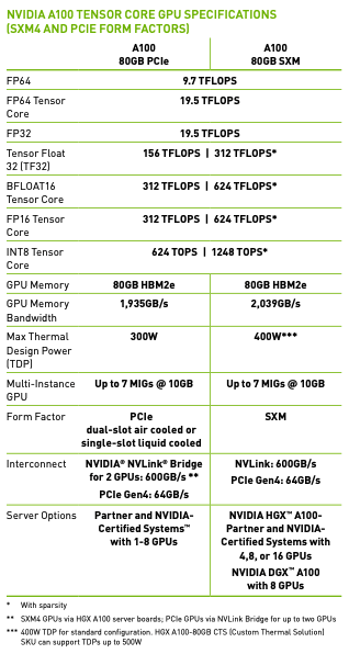
Understanding the GPU datasheet: The above table is from the datasheet. It is split into several sections. The first part is the number of operations the GPU can handle per second (units of TFLOPs indicate how many millions of floating point calculations per second the GPU can do). By default PyTorch tensors are in float32. That means all the activations, weights, and so on use float32. That means each number is using 32 bits of memory. That is a lot of memory for each number and it turns out certain workloads like machine learning can suffice with less precise numbers like bfloat32. If you look at the row for FP32, it says 19.5 TFLOPS. That means you can expect this GPU to do 19.5 trillion operations per second (operations as in floating point addition or multiplication most commonly). You can see that if you are willing to drop to a lower precision datatype, then the TFLOPS you can expect your GPU to perform goes up. A couple of notes: the numbers with the single asterisk (*) are the TFLOPS with Sparsity, but we won't be using that and generally people in industry don't use sparsity. Also you might notice that under FP16 there is INT8. INT8 is used for inference time, but because we are training we need floating point numbers. Because these numbers take less bits, it's also easier to move them around. That's when we get into the memory and memory bandwidth of the model. Not only is there a finite amount of bits that can be stored on this GPU (for my A100 it would be 80GB), but also there is a cap on the speed you can access these bits (1935 GB/s). This bandwidth is a very precious resource. In fact the machine learning workloads are often "memory bound": these GPUs are idle because we can't feed the GPU's smaller parts (called tensor cores, we'll get to that soon) fast enough. When we decrease the numbers precision, we can store more and we can access it faster (because there is a cap on the memory and memory bandwidth of the GPUs). Let's reap the benefits of going to a lower precision!
Tensor cores: Before that, let's understand what tensor cores are. "Tensor cores" are instructions in the A100 architecture. Specifically it's a multiplication between 2 four by four matrices (oversimplified explanation; after the multiplication there is also an addition called the "accumulation"). Whenever we want to do a dot product in our code, it gets broken up into these tensor core instructions. Most of the work we are doing while training is matrix multiplies. Most of the work is being done in the linear layers. There are some additions and nonlinearities and layer norms, etc., but if you look at how much time each operation takes the vast majority of time is taken up by matrix multiplies. The biggest matrix multiply is actually the top classifier going from 768 (n_embd) to 50257 (vocab size). This is why sharing the embedding layer and the lm_head linear layer was so efficient.
So how does TF32 work? The inputs, the accumulation (which is the hidden addition I mentioned in a tensor core operation), and the outputs are all still floating point 32. The inputs get converted to the TF32 data type (where some of the mantissa bits are truncated), the operation happens, and then the data is converted back into FP32 for the accumulation and output. Why do all of this conversion? Remember if you go back to the above table we get almost an 8X speedup if we use TF32 over FP32 theoretically. But empirically you basically can't tell the difference. So if your workload can handle the slight precision loss, this is basically a "free" speedup. Let's test this in our setup. Here is the speed and throughput for each epoch with FP32:
(venv) oagrawal@mew3:/nfs/oagrawal/andrej/build-nanogpt$ python3 train_gpt2.py
using device: cuda
loaded 338025 tokens
1 epoch = 20 batches
step 0, loss: 10.935506820678711, dt: 2006.43ms, tok/sec: 8165.74
step 1, loss: 9.398406982421875, dt: 1279.08ms, tok/sec: 12809.16
step 2, loss: 8.941734313964844, dt: 1279.09ms, tok/sec: 12809.15
step 3, loss: 8.818683624267578, dt: 1279.04ms, tok/sec: 12809.65
step 4, loss: 8.487004280090332, dt: 1278.70ms, tok/sec: 12812.99
step 5, loss: 8.465452194213867, dt: 1279.04ms, tok/sec: 12809.64
step 6, loss: 8.293403625488281, dt: 1279.42ms, tok/sec: 12805.83
step 7, loss: 8.081167221069336, dt: 1278.85ms, tok/sec: 12811.46
step 8, loss: 7.802502632141113, dt: 1345.48ms, tok/sec: 12177.10
Here is the speed and throughput with TF32:
(venv) oagrawal@mew3:/nfs/oagrawal/andrej/build-nanogpt$ python3 train_gpt2.py
using device: cuda
loaded 338025 tokens
1 epoch = 20 batches
step 0, loss: 10.935468673706055, dt: 980.16ms, tok/sec: 16715.60
step 1, loss: 9.398319244384766, dt: 386.64ms, tok/sec: 42375.17
step 2, loss: 8.94157886505127, dt: 386.97ms, tok/sec: 42339.56
step 3, loss: 8.818317413330078, dt: 387.16ms, tok/sec: 42318.86
step 4, loss: 8.486916542053223, dt: 386.93ms, tok/sec: 42343.71
step 5, loss: 8.465150833129883, dt: 387.11ms, tok/sec: 42323.65
step 6, loss: 8.29329776763916, dt: 387.02ms, tok/sec: 42333.80
step 7, loss: 8.081138610839844, dt: 387.04ms, tok/sec: 42331.87
step 8, loss: 7.802093505859375, dt: 386.96ms, tok/sec: 42340.60
There is roughly a 3.5X speedup we get essentially "for free" (there is very slight precision degradation, almost unnoticeable). To change set the following line:
torch.set_float32_matmul_precision('high')Where "highest" is FP32 and "high" is TF32. Why are we only getting a 3.5X speedup though? Shouldn't it be 8X? That is correct. The reason is because this workload is memory bound, and we aren't able to fully utilize the GPUs. More specifically, although the precision used in the tensor core underlying multiplication is lower, the input and outputs are still FP32, and so we are still shipping FP32 numbers around! This is a memory bottleneck, and we will need to somehow get the data to the GPUs faster so that they can get closer to their full speedup potential. We can do this by reducing the precision of the actual datatype, so we can get more of these numbers to the GPU in the same time.
Let's drop down to the BFLOAT16 data type! We will only maintain 16 bits per float. Essentially compared to TF32, we still have the same sign bit and the exponent bits, but we reduce the number of mantissa bits. This means we can still express the full range we had with TF32, except the precision will be a little more degraded. There was a middle ground between TF32 and BFLOAT16 called FP16, but what that does is reduce the exponent range, so people had to use gradient scalars to get the full range. Thankfully now with the Ampere series of GPUs we can do BFLOAT16, and the full range of the numbers is still intact so we don't have to mess around with gradient scalars and such. But unlike the change from FP32 to TF32 where the change was local, from TF32 to BFLOAT16 we are impacting the numbers. So this change is not just local to the tensor core operations: we might be impacting other operations as well. To change from TF32 to BFLOAT16, we do the following change:
optimizer = torch.optim.AdamW(model.parameters(), lr=3e-4)
for i in range(50):
    t0 = time.time()
    x, y = train_loader.next_batch()
    x, y = x.to(device), y.to(device)
    optimizer.zero_grad()
    with torch.autocast(device_type=device, dtype=torch.bfloat16):
        logits, loss = model(x, y)
    loss.backward()
    optimizer.step()
    torch.cuda.synchronize()  # wait for the GPU to finish work
    t1 = time.time()
    dt = (t1 - t0)*1000  # time difference in milliseconds
    tokens_per_sec = (train_loader.B * train_loader.T) / (t1 - t0)
    print(f"step {i}, loss: {loss.item()}, dt: {dt:.2f}ms, tok/sec: {tokens_per_sec:.2f}")
Let's run our optimization again and see the time between epochs and the throughput:
(venv) oagrawal@mew3:/nfs/oagrawal/andrej/build-nanogpt$ python3 train_gpt2.py
using device: cuda
loaded 338025 tokens
1 epoch = 20 batches
step 0, loss: 10.936103820800781, dt: 1163.31ms, tok/sec: 14083.98
step 1, loss: 9.398155212402344, dt: 343.70ms, tok/sec: 47669.03
step 2, loss: 8.943115234375, dt: 343.68ms, tok/sec: 47671.70
step 3, loss: 8.822978019714355, dt: 343.90ms, tok/sec: 47642.26
step 4, loss: 8.487868309020996, dt: 343.64ms, tok/sec: 47677.16
step 5, loss: 8.469024658203125, dt: 343.69ms, tok/sec: 47671.11
step 6, loss: 8.294583320617676, dt: 343.58ms, tok/sec: 47685.50
step 7, loss: 8.081433296203613, dt: 343.65ms, tok/sec: 47676.43
step 8, loss: 7.805779457092285, dt: 344.12ms, tok/sec: 47611.62
step 9, loss: 7.5632476806640625, dt: 343.62ms, tok/sec: 47680.17
step 10, loss: 7.397215843200684, dt: 343.66ms, tok/sec: 47675.44
As we can see there is a speedup and the throughput went up. That's it! With this context manager we have the forward pass of the model and the loss calculation in the autocast. I would like to highlight that this has changed the datatype of the logits to bfloat16 (unlike when we went from FP32 to TF32 everything was still FP32). But not everything has changed: our parameters are still in FP32, but activations are in BFLOAT16. Hence the name mixed precision (AMP). In the PyTorch docs, the multiplication type operations get converted to BFLOAT16, and the rest get converted to float32 (e.g. layer norms, softmax, loss function calculations). These layers/calculations that remain in FP32 remain in this format because they are more susceptible to degradations due to less precision.
Now let's use some more powerful tools at our disposal to speed things up. There is a tool called torch.compile. This is also just a one line change to our codebase, but while it slows down the one time compilation, each epoch takes less time.
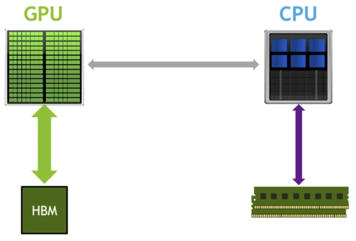
What does torch.compile do? Let's look at the above GPU architecture mental model (on the left is GPU cores and memory (HBM), on the right is the CPU and RAM). One thing it does is remove the python interpreter from the equation. Regularly when we are running optimization with our model, Python goes line by line, looks at the command and calls kernels, etc. in a lazy fashion. It doesn't know anything about what the future calls will be. This is not optimal because the code should know what the future calls will be. It is literally defined in the GPT class! So torch.compile looks at the entire torch codebase at once, and optimizes things based off of what will be in the future (because it knows the order of what commands run after what), and removes the python interpreter from the picture. The second thing it does is optimize GPU cores to GPU memory trips. For example, suppose we are doing a GELU nonlinearity. This nonlinearity has a bunch of operations on the same data. There can be element wise multiplication, element wise addition, etc. For each of these such operations, without torch.compile we would move data from GPU memory to GPU cores, do the operation, write back to GPU memory. For the next operation we do the same: move the data from GPU memory to GPU cores, do the operation, and write back to GPU memory. You can see how this is inefficient. We know we are doing an element wise operation (for example), so instead of writing back to GPU memory right before we will need to read that same data back into the GPU cores, how about we just keep the data in the GPU cores and do all of the operations (if we have kernel fusion) before writing back to the GPU memory. Without torch.compile we couldn't do this because we don't have access to what future commands will be. But with torch.compile, because this tool looks at the entire codefile as a snapshot, we do know the future commands that will follow certain commands. This optimizes GPU memory to GPU core trips, and saves us a lot on the critical resource of GPU memory bandwidth.
Here are the epoch times now:
(venv) oagrawal@mew3:/nfs/oagrawal/andrej/build-nanogpt$ python3 train_gpt2.py
using device: cuda
loaded 338025 tokens
1 epoch = 20 batches
step 0, loss: 10.935912132263184, dt: 34843.30ms, tok/sec: 470.22
step 1, loss: 9.398194313049316, dt: 150.26ms, tok/sec: 109035.27
step 2, loss: 8.942642211914062, dt: 149.56ms, tok/sec: 109550.12
step 3, loss: 8.822107315063477, dt: 149.49ms, tok/sec: 109602.54
step 4, loss: 8.487815856933594, dt: 149.54ms, tok/sec: 109565.67
step 5, loss: 8.468069076538086, dt: 149.56ms, tok/sec: 109549.42
step 6, loss: 8.294349670410156, dt: 149.44ms, tok/sec: 109632.61
step 7, loss: 8.08154582977295, dt: 149.48ms, tok/sec: 109605.69
step 8, loss: 7.805381774902344, dt: 149.51ms, tok/sec: 109585.06
step 9, loss: 7.563920021057129, dt: 149.50ms, tok/sec: 109589.60
step 10, loss: 7.396984100341797, dt: 149.21ms, tok/sec: 109808.32
This is a decent amount of speedup over just BFLOAT16, a 2.3x speedup. Torch.compile is amazing, but it doesn't find all optimizations and kernel fusions. One such example of this is flash attention, which fuses the following 4 lines in the self attention into one fused kernel:
att = (q @ k.transpose(-2, -1)) * (1.0 / math.sqrt(k.size(-1)))
att = att.masked_fill(self.bias[:,:,:T,:T] == 0, float('-inf'))
att = F.softmax(att, dim=-1)
y = att @ v  # (B, nh, T, T) x (B, nh, T, hs) -> (B, nh, T, hs)
Why doesn't torch.compile find the flash attention fusion? Because to get this optimization you have to rewrite the algorithm. What's remarkable is flash attention does more FLOPS than the 4 lines above. But because flash attention is very mindful of the memory hierarchy present in GPUs such that there are fewer reads and writes to the HBM, this results in a 7.6x speedup for attention. What is the idea with flash attention? To never materialize the NxN affinities matrix. The way they never materialize the nxn matrix of affinities is by implementing softmax in an online fashion (that doesn't require having all the inputs; instead you can get the result of the softmax just by having a subset of inputs and updating the softmax result as you get more of the inputs). Let's use flash attention. Here is the one line we can use to replace the above 4 lines:
y = F.scaled_dot_product_attention(q, k, v, is_causal=True) # flash attentionLet's see what the epoch times are now:
(venv) oagrawal@mew3:/nfs/oagrawal/andrej/build-nanogpt$ python3 train_gpt2.py
using device: cuda
loaded 338025 tokens
1 epoch = 20 batches
step 0, loss: 10.93594741821289, dt: 22511.02ms, tok/sec: 727.82
step 1, loss: 9.398148536682129, dt: 114.08ms, tok/sec: 143623.98
step 2, loss: 8.942426681518555, dt: 113.39ms, tok/sec: 144496.75
step 3, loss: 8.820838928222656, dt: 113.69ms, tok/sec: 144115.54
step 4, loss: 8.487611770629883, dt: 113.55ms, tok/sec: 144286.81
step 5, loss: 8.467279434204102, dt: 113.70ms, tok/sec: 144098.01
step 6, loss: 8.294020652770996, dt: 114.05ms, tok/sec: 143661.81
step 7, loss: 8.081624031066895, dt: 113.82ms, tok/sec: 143945.58
step 8, loss: 7.804403305053711, dt: 113.62ms, tok/sec: 144195.98
step 9, loss: 7.563755035400391, dt: 113.67ms, tok/sec: 144140.63
This is a 1.3x speedup just by this one fused kernel! The next improvement is a dumb yet brilliant optimization: it is to scan your code for ugly numbers and change them to nice numbers. By ugly I just mean non power of two numbers or prime numbers or odd numbers, whereas nice numbers are even, power of two, etc. The reason this could lead to a speedup is a lot of things in CUDA are optimized for power of two groupings (e.g. maybe the number of cores are a power of two). If we scan through the code we see that one extremely non nice number is the vocab size of 50257. Let's change this to a close yet large number 50304. What we are essentially doing here is adding extra tokens. By doing this, we are also increasing the number of flops, but let's see what effect this has on our epoch times:
(venv) oagrawal@mew3:/nfs/oagrawal/andrej/build-nanogpt$ python3 train_gpt2.py
using device: cuda
loaded 338025 tokens
1 epoch = 20 batches
step 0, loss: 10.947359085083008, dt: 20391.03ms, tok/sec: 803.49
step 1, loss: 9.388193130493164, dt: 110.72ms, tok/sec: 147977.31
step 2, loss: 8.963235855102539, dt: 109.96ms, tok/sec: 148998.56
step 3, loss: 8.852298736572266, dt: 110.05ms, tok/sec: 148871.70
step 4, loss: 8.50532341003418, dt: 109.83ms, tok/sec: 149177.10
step 5, loss: 8.47411060333252, dt: 109.98ms, tok/sec: 148975.95
step 6, loss: 8.318906784057617, dt: 109.86ms, tok/sec: 149129.19
step 7, loss: 8.0703706741333, dt: 109.98ms, tok/sec: 148979.18
step 8, loss: 7.814784049987793, dt: 110.07ms, tok/sec: 148854.61
step 9, loss: 7.591421127319336, dt: 110.06ms, tok/sec: 148866.87
step 10, loss: 7.390069007873535, dt: 109.82ms, tok/sec: 149192.00
We see that this simple "optimization" gives us a 2 to 3 percent speedup! How crazy is that.
Section 3: Algorithmic Improvements
At this point we have a roughly 11x speedup over the original non optimized training algorithm. We are doing a much better job of using our GPU resources. Now we would like to turn to algorithmic improvements: improvement to the actual optimization itself, following the hyperparameters in the GPT 2 and GPT 3 papers. We look into the GPT 2 paper, but while they do release their code and weights they omit a lot of details regarding the pretraining process. Thankfully the GPT 3 paper has more details about the training process, albeit they don't release weights.
Here are the AdamW hyperparameters from the GPT2 paper:
optimizer = torch.optim.AdamW(model.parameters(), lr=3e-4, betas=(0.9, 0.95), eps=1e-8)They also mention they clip the global norm of the gradient at 1.0. The global norm is: for each parameter in the network we square the value, add it all up, and take the square root of this. We want to make sure this value is 1.0. The reason people do this is during training you can have a mini batch that has bad data. This bad data can lead to a high loss, which can lead to a high gradient, which can "shock" your model. You don't want this shock during the optimization, which is why people clip the gradient like this. We will also print this norm value during optimization steps. This is a good idea because if the norm is increasing or suddenly has a spike then there is some sort of instability during training. They also use a cosine decay learning rate (decay of 10% over a horizon). The following is a visualization of the learning rate decay:
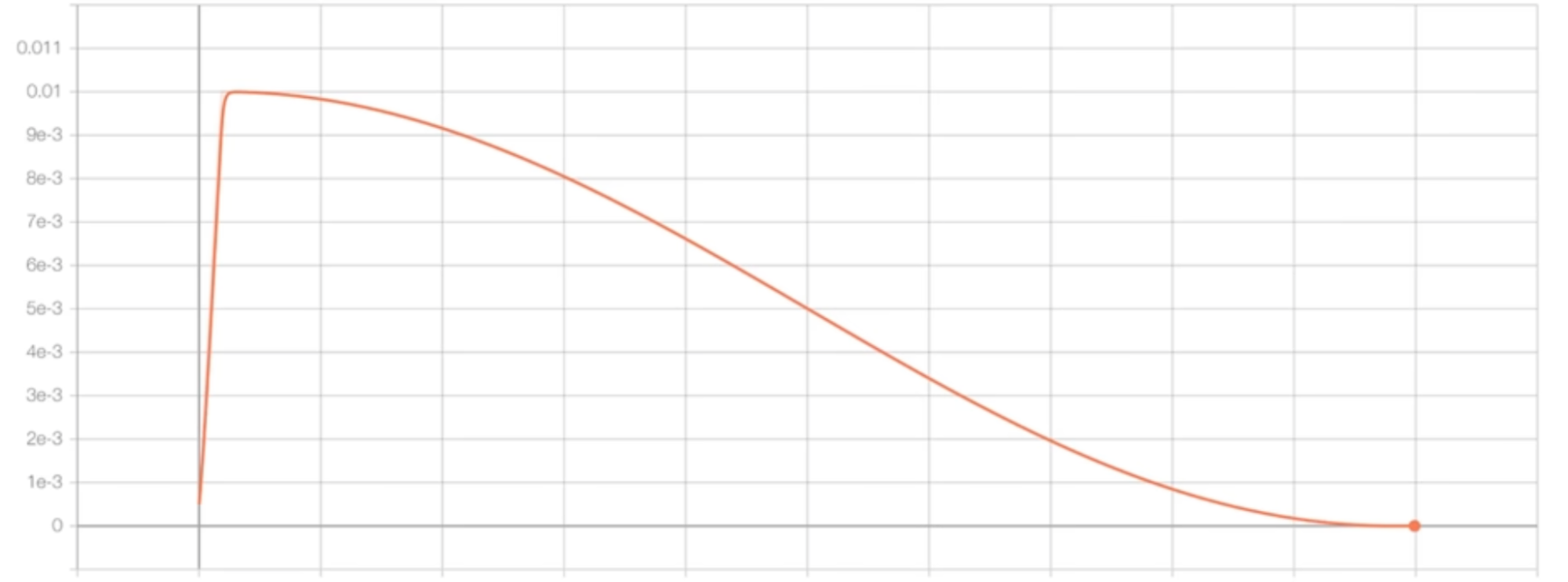
The learning rate linearly increases, then after that short horizon it decays according to a cosine function. This learning rate schedule is implemented as the following:
max_lr = 6e-4
min_lr = max_lr * 0.1
warmup_steps = 10
max_steps = 50
def get_lr(it):
    # 1) linear warmup for warmup_iters steps
    if it < warmup_steps:
        return max_lr * (it+1) / warmup_steps
    # 2) if it > lr_decay_iters, return min learning rate
    if it > max_steps:
        return min_lr
    # 3) in between, use cosine decay down to min learning rate
    decay_ratio = (it - warmup_steps) / (max_steps - warmup_steps)
    assert 0 <= decay_ratio <= 1
    coeff = 0.5 * (1.0 + math.cos(math.pi * decay_ratio))  # coeff starts at 1 and goes to 0
    return min_lr + coeff * (max_lr - min_lr)
And this is how you can add it to the optimization loop: set lr = get_lr(step) and update param_group['lr'] before optimizer.step(). The GPT paper also mentions that they start with a small batch size and linearly increase the batch size. We won't be following this because this complicates the arithmetic of the training. We currently are processing the same number of tokens for each step, but with this change we would be changing the number of tokens processed on each step. We will skip this optimization. It is more of an efficiency optimization too rather than a correctness optimization. For sampling data for mini batches for training, they are doing so without replacement. We are already doing this. Our data loader iterates over chunks of data, and once a chunk is sampled it cannot be sampled again until the next epoch. GPT 3 also uses a weight decay of 0.1. Let's change our optimizer object to match this:
optimizer = model.configure_optimizers(weight_decay=0.1, learning_rate=6e-4, device=device)Where model.configure_optimizers is:
def configure_optimizers(self, weight_decay, learning_rate, device):
    # start with all of the candidate parameters (that require grad)
    param_dict = {pn: p for pn, p in self.named_parameters()}
    param_dict = {pn: p for pn, p in param_dict.items() if p.requires_grad}
    # create optim groups. Any parameters that is 2D will be weight decayed, otherwise no.
    # i.e. all weight tensors in matmuls + embeddings decay, all biases and layernorms don't.
    decay_params = [p for n, p in param_dict.items() if p.dim() >= 2]
    nodecay_params = [p for n, p in param_dict.items() if p.dim() < 2]
    optim_groups = [
        {'params': decay_params, 'weight_decay': weight_decay},
        {'params': nodecay_params, 'weight_decay': 0.0}
    ]
    num_decay_params = sum(p.numel() for p in decay_params)
    num_nodecay_params = sum(p.numel() for p in nodecay_params)
    print(f"num decayed parameter tensors: {len(decay_params)}, with {num_decay_params:,} parameters")
    print(f"num non-decayed parameter tensors: {len(nodecay_params)}, with {num_nodecay_params:,} parameters")
    # Create AdamW optimizer and use the fused version if it is available
    fused_available = 'fused' in inspect.signature(torch.optim.AdamW).parameters
    use_fused = fused_available and 'cuda' in device
    print(f"using fused AdamW: {use_fused}")
    optimizer = torch.optim.AdamW(optim_groups, lr=learning_rate, betas=(0.9, 0.95), eps=1e-8, fused=use_fused)
    return optimizer
This looks very complicated but it is in reality pretty simple. Andrej here is splitting the parameters into those which should and should not be affected by weight decay. It is common to not weight decay biases and any other one dimensional tensors (also scales, layer norms, biases). You generally do want to weight decay the weights that participate in matrix multiplications and embeddings. This weight decay prevents any one feature from dominating, which forces the model to "spread" its learning to all of the features. It acts like a regularization technique. You can implement this by adding a penalty term to the loss function based on the size of the weights. There is an additional optimization: the fused AdamW kernel. Essentially in older versions of PyTorch they had to iteratively run the optimizer, but recently PyTorch came out with a fused kernel to run the optimization at once instead of iteratively. Recall this is what a fused kernel does. This optimization is essentially a fused kernel for the AdamW optimizer. It runs much faster. Let's run our training script after implementing these details from the GPT 3 paper:
(venv) oagrawal@mew3:/nfs/oagrawal/andrej/build-nanogpt$ python3 train_gpt2.py
using device: cuda
loaded 338025 tokens
1 epoch = 20 batches
num decayed parameter tensors: 50, with 124,354,560 parameters
num non-decayed parameter tensors: 98, with 121,344 parameters
using fused AdamW: True
step    0 | loss: 10.947359 | lr 6.0000e-05 | norm: 28.5683 | dt: 5243.63ms | tok/sec: 3124.56
step    1 | loss: 9.502396 | lr 1.2000e-04 | norm: 10.6571 | dt: 108.74ms | tok/sec: 150664.92
step    2 | loss: 9.251488 | lr 1.8000e-04 | norm: 7.3693 | dt: 107.50ms | tok/sec: 152410.88
step    3 | loss: 9.762377 | lr 2.4000e-04 | norm: 6.6550 | dt: 107.54ms | tok/sec: 152350.40
step    4 | loss: 9.105073 | lr 3.0000e-04 | norm: 4.2452 | dt: 107.14ms | tok/sec: 152927.79
step    5 | loss: 8.795052 | lr 3.6000e-04 | norm: 3.2618 | dt: 106.81ms | tok/sec: 153387.58
step    6 | loss: 8.586094 | lr 4.2000e-04 | norm: 2.3601 | dt: 106.75ms | tok/sec: 153484.53
step    7 | loss: 8.265682 | lr 4.8000e-04 | norm: 2.0499 | dt: 106.84ms | tok/sec: 153350.96
step    8 | loss: 7.888580 | lr 5.4000e-04 | norm: 2.2143 | dt: 107.00ms | tok/sec: 153127.82
As you can see, there are a lot more decayed parameters compared to non-decayed parameters. We are also using fused AdamW, which might be why we are getting some slight speedups compared to the last training configuration we were using.
We are essentially copy pasting these hyperparameters from the GPT2/GPT3 papers, but these hyperparameters are all highly correlated according to complex optimization math. We won't be doing a deep dive into this field in this blog post, but just want to put that idea out there. Because if we go back to see what the batch size GPT 3 small used, it is 0.5M (tokens). That is roughly 500,000 / 1024 = 488 items in a batch. The problem is that we can't just substitute 488 for B. 488 batches each of 1024 will definitely not fit in our one GPU. But we still have to use this same batch size (because all of the other hyperparameters in the optimization are correlated to this batch size). So how can we proceed? How can we fit this large batch size onto our GPU setup? We can use a technique called gradient accumulation. Gradient accumulation allows us to simulate larger batch sizes serially, and to do this we will need to add up gradients. Which is why this technique is called gradient accumulation.
So the total batch size we want is total_batch_size = 524288 (2**19, approximately 0.5M, in number of tokens). We choose this number because it is a nice number (power of two!). Our micro batch size, as we'll call it now, is 16, and our sequence length is 1024. The mental model I want you to have for gradient accumulation is we will still have these forward passes, loss, and backward passes to calculate the gradients. But we will not update the weights yet. We will keep running this forward and backward passes until we've reached the total batch size we are trying to simulate, keep adding (plus equals) the gradients, and then finally at the end of this simulated batch we will update our weights. In this case batch size is 2**19, and our micro batch size is 16 microbatches times 1024 tokens for each microbatch equals 16384. That means that we will have 2**19 / (16 * 1024) = 32 forward + backward passes of our microbatches until we hit our larger batch size. This means that because our previous training config took approximately 100ms per "microbatch", our total batch will take 32 times that, or around 3.2 seconds per actual batch.
Here is our optimization loop with our micro batches:
optimizer = model.configure_optimizers(weight_decay=0.1, learning_rate=6e-4, device=device)

for step in range(max_steps):
    t0 = time.time()
    optimizer.zero_grad()
    loss_accum = 0.0
    for micro_step in range(grad_accum_steps):
        x, y = train_loader.next_batch()
        x, y = x.to(device), y.to(device)
        with torch.autocast(device_type=device, dtype=torch.bfloat16):
            logits, loss = model(x, y)
        # we have to scale the loss to account for gradient accumulation,
        # because the gradients just add on each successive backward().
        # addition of gradients corresponds to a SUM in the objective, but
        # instead of a SUM we want MEAN. Scale the loss here so it comes out right
        loss = loss / grad_accum_steps
        loss_accum += loss.detach()
        loss.backward()
    norm = torch.nn.utils.clip_grad_norm_(model.parameters(), 1.0)
    lr = get_lr(step)
    for param_group in optimizer.param_groups:
        param_group['lr'] = lr
    optimizer.step()
    torch.cuda.synchronize()
    t1 = time.time()
    dt = t1 - t0
    tokens_processed = train_loader.B * train_loader.T * grad_accum_steps
    tokens_per_sec = tokens_processed / dt
    print(f"step {step:4d} | loss: {loss_accum.item():.6f} | lr {lr:.4e} | norm: {norm:.4f} | dt: {dt*1000:.2f}ms | tok/sec: {tokens_per_sec:.2f}")
The "loss = loss / grad_accum_steps" is quite subtle. If we didn't divide the loss by the number of microbatches, then we keep increasing the gradient as we run more microbatches. This would cause our gradient to be different than the same examples run in a batch. Instead, what we want is for each gradient to be averaged across the number of batch examples. One way we can implement this is by dividing the loss by the number of microbatches. Once we've implemented gradient accumulation, here is our optimization output. As expected dt is around 3.2 seconds per batch:
(venv) oagrawal@mew3:/nfs/oagrawal/andrej/build-nanogpt$ python3 train_gpt2.py
using device: cuda
total desired batch size: 524288
=> calculated gradient accumulation steps: 32
loaded 338025 tokens
1 epoch = 20 batches
num decayed parameter tensors: 50, with 124,354,560 parameters
num non-decayed parameter tensors: 98, with 121,344 parameters
using fused AdamW: True
step    0 | loss: 10.938565 | lr 6.0000e-05 | norm: 27.0126 | dt: 6078.27ms | tok/sec: 86256.14
step    1 | loss: 9.649337 | lr 1.2000e-04 | norm: 9.5176 | dt: 3348.29ms | tok/sec: 156583.80
step    2 | loss: 9.225615 | lr 1.8000e-04 | norm: 5.7295 | dt: 3349.83ms | tok/sec: 156511.96
step    3 | loss: 9.813120 | lr 2.4000e-04 | norm: 8.2064 | dt: 3369.35ms | tok/sec: 155605.10
step    4 | loss: 9.191647 | lr 3.0000e-04 | norm: 4.2994 | dt: 3370.01ms | tok/sec: 155574.67
step    5 | loss: 8.678038 | lr 3.6000e-04 | norm: 3.6286 | dt: 3369.25ms | tok/sec: 155609.88
step    6 | loss: 8.294975 | lr 4.2000e-04 | norm: 1.9535 | dt: 3369.87ms | tok/sec: 155581.01
step    7 | loss: 8.068053 | lr 4.8000e-04 | norm: 2.8529 | dt: 3368.63ms | tok/sec: 155638.49
step    8 | loss: 7.714221 | lr 5.4000e-04 | norm: 1.9106 | dt: 3366.09ms | tok/sec: 155756.02
step    9 | loss: 7.347071 | lr 6.0000e-04 | norm: 1.8007 | dt: 3365.89ms | tok/sec: 155765.21
step   10 | loss: 7.029751 | lr 6.0000e-04 | norm: 1.8395 | dt: 3366.57ms | tok/sec: 155733.49
step   11 | loss: 6.741249 | lr 5.9917e-04 | norm: 1.5063 | dt: 3364.95ms | tok/sec: 155808.37
DistributedDataParallel
Andrej has more than 1 GPU on the machine, but is only using 1 GPU. How can he use all of the GPUs to make progress? One answer is DistributedDataParallel (DDP). With DDP we will be launching the same number of processes as we have GPUs. For each process the training loop looks the same, except for each process they will be training on different data. Another change: when each process calculates the gradient for each parameter, we actually average the gradient across the GPUs. That's how they will be collaborating on the workload.
To use DistributedDataParallel, instead of running python3 train_gpt2.py, we will run a special command called torchrun. When we run using torchrun, our train script will be run in parallel on as many processes as there are GPUs. Torchrun will create these variables such that each process knows which process it is out of the total processes that are processing all of the data in parallel. We will mainly be interested in RANK and WORLD_SIZE. WORLD_SIZE is the number of processes running, and RANK is what process you are in. Here is that spelled out in code:
ddp = int(os.environ.get('RANK', -1)) != -1  # is this a ddp run?
if ddp:
    assert torch.cuda.is_available(), "for now i think we need CUDA for DDP"
    init_process_group(backend='nccl')
    ddp_rank = int(os.environ['RANK'])
    ddp_local_rank = int(os.environ['LOCAL_RANK'])
    ddp_world_size = int(os.environ['WORLD_SIZE'])
    device = f'cuda:{ddp_local_rank}'
    torch.cuda.set_device(device)
    master_process = ddp_rank == 0  # this process will do logging, checkpointing etc.
else:
    ddp_rank = 0
    ddp_local_rank = 0
    ddp_world_size = 1
    master_process = True
To write programs that have functionality dependent on which GPU you are (e.g. reading a specific part of the input depending on which GPU you are), you can use the RANK environment variable. Previously with gradient accumulation we had 32 microbatches. But now that we have WORLD_SIZE processes (e.g. 4 GPUs), it will take us 2**19 / (16 * 1024 * 4) = 8 microbatches to complete a batch. You might have also noticed that we calculate a "master process". This is an arbitrarily chosen process that will do all of our prints. If we don't set this then all of the processes will print, which will lead to very confusing print statements. Next we edit the dataloader to make it aware of this multiprocess setting. Specifically we want each rank to get their own chunk of data:
class DataLoaderLite:
    def __init__(self, B, T, process_rank, num_processes):
        self.B = B
        self.T = T
        self.process_rank = process_rank
        self.num_processes = num_processes
        with open('input.txt', 'r') as f:
            text = f.read()
        enc = tiktoken.get_encoding('gpt2')
        tokens = enc.encode(text)
        self.tokens = torch.tensor(tokens)
        if master_process:
            print(f"loaded {len(self.tokens)} tokens")
        self.current_position = self.B * self.T * self.process_rank

    def next_batch(self):
        B, T = self.B, self.T
        buf = self.tokens[self.current_position : self.current_position+B*T+1]
        x = (buf[:-1]).view(B, T)
        y = (buf[1:]).view(B, T)
        self.current_position += B * T * self.num_processes
        if self.current_position + (B * T * self.num_processes + 1) > len(self.tokens):
            self.current_position = self.B * self.T * self.process_rank
        return x, y
Essentially we are striding where each RANK starts loading data from. Once that rank finishes processing the B*T tokens, instead of going to the next B*T tokens (which must have been assigned to a different GPU if WORLD_SIZE > 1) we advance the current_position by B*T*WORLD_SIZE. Next up, once the dataloaders are initialized for each RANK, they each initialize the GPT model. Each process then wraps their model in the DDP object. What DDP does is, on the backward pass once the gradient is calculated for each process, it averages the gradients and sets the gradients of all ranks to be this average gradient vector. It implements this using AllReduce. DDP overlaps computation and communication. By default when you call loss.backward(), gradient synchronization will happen. Because of gradient accumulation we call loss.backward() after every microbatch. With DDP we don't want to synchronize after every microbatch; we just want to synchronize the gradients at the last microbatch. The official way to do this is using a no_sync() context manager, but Andrej prefers directly setting model.require_backward_grad_sync = False for all microsteps except the last one, and True for the last microbatch. There is still a problem: loss_accum only accumulated the losses that the current rank has seen. We want the average loss across all processes. After the microbatch loop we call dist.all_reduce(loss_accum, op=dist.ReduceOp.AVG). Finally we want to call destroy_process_group() so that we exit from each process cleanly.
Alright, with DDP let's see what our optimization output looks like:
(venv) oagrawal@mew2:/nfs/oagrawal/andrej/build-nanogpt$ torchrun --standalone --nproc_per_node=4 train_gpt2.py
W0315 22:18:19.385000 2714186 torch/distributed/run.py:852]
W0315 22:18:19.385000 2714186 torch/distributed/run.py:852] *****************************************
W0315 22:18:19.385000 2714186 torch/distributed/run.py:852] Setting OMP_NUM_THREADS environment variable for each process to be 1 in default, to avoid your system being overloaded, please further tune the variable for optimal performance in your application as needed.
W0315 22:18:19.385000 2714186 torch/distributed/run.py:852] *****************************************
total desired batch size: 524288
=> calculated gradient accumulation steps: 8
loaded 338025 tokens
num decayed parameter tensors: 50, with 124,354,560 parameters
num non-decayed parameter tensors: 98, with 121,344 parameters
using fused AdamW: True
step    0 | loss: 10.938540 | lr 6.0000e-05 | norm: 27.8107 | dt: 20964.03ms | tok/sec: 25008.94
step    1 | loss: 9.658166 | lr 1.2000e-04 | norm: 9.5822 | dt: 770.45ms | tok/sec: 680492.34
step    2 | loss: 9.207886 | lr 1.8000e-04 | norm: 5.9203 | dt: 768.09ms | tok/sec: 682587.73
step    3 | loss: 9.802918 | lr 2.4000e-04 | norm: 8.0720 | dt: 768.72ms | tok/sec: 682030.73
step    4 | loss: 9.181516 | lr 3.0000e-04 | norm: 4.3056 | dt: 768.67ms | tok/sec: 682069.02
step    5 | loss: 8.652848 | lr 3.6000e-04 | norm: 3.6443 | dt: 766.90ms | tok/sec: 683644.09
step    6 | loss: 8.295362 | lr 4.2000e-04 | norm: 1.9758 | dt: 766.61ms | tok/sec: 683908.16
step    7 | loss: 8.017211 | lr 4.8000e-04 | norm: 2.5486 | dt: 766.62ms | tok/sec: 683891.78
step    8 | loss: 7.672647 | lr 5.4000e-04 | norm: 1.9825 | dt: 766.16ms | tok/sec: 684304.01
step    9 | loss: 7.301464 | lr 6.0000e-04 | norm: 1.8976 | dt: 767.87ms | tok/sec: 682784.83
step   10 | loss: 6.959521 | lr 6.0000e-04 | norm: 1.7909 | dt: 770.30ms | tok/sec: 680625.88
step   11 | loss: 6.670654 | lr 5.9917e-04 | norm: 1.3795 | dt: 772.53ms | tok/sec: 678660.82
...
step   47 | loss: 5.681354 | lr 6.7460e-05 | norm: 0.2736 | dt: 787.56ms | tok/sec: 665711.83
step   48 | loss: 5.675771 | lr 6.3324e-05 | norm: 0.2083 | dt: 788.62ms | tok/sec: 664813.41
step   49 | loss: 5.675558 | lr 6.0832e-05 | norm: 0.1775 | dt: 788.06ms | tok/sec: 665287.68
Bigger Dataset
We have outgrown our Tiny Shakespeare file. Let's get some bigger datasets. GPT 2 created an unreleased dataset called WebText by scraping all outbound links from Reddit which received at least 3 karma. This was 40GB of text. GPT 3 used CommonCrawl. It's much more used but it's not a very high quality dataset, much worse than you think. People like to filter this. That's why people like to train on data mixtures that they curate: large chunk can be CommonCrawl, WebText2 (Reddit outbound), books, Wikipedia. Nowadays there are pretty good open source datasets: RedPajama (specifically the SlimPajama dataset), FineWeb (really high quality CommonCrawl filtered data), FineWeb Edu subset (from Hugging Face, very high quality educational subset of FineWeb dataset). We will be working with FineWeb Edu, specifically the sample-10B token subset. We use fineweb.py to download, tokenize (start with <endoftext> special token + rest of tokens, save as np.uint16 shards of 100M tokens each). We run approximately 19,073 steps for 10B tokens, warmup over 375M tokens, batch size 64.
Here are the early steps when we start the FineWeb pretraining run:
(venv) oagrawal@mew2:/nfs/oagrawal/andrej/build-nanogpt$ torchrun --standalone --nproc_per_node=4 train_gpt2.py
W0316 00:40:13.550000 2817223 torch/distributed/run.py:852]
W0316 00:40:13.550000 2817223 torch/distributed/run.py:852] *****************************************
W0316 00:40:13.550000 2817223 torch/distributed/run.py:852] Setting OMP_NUM_THREADS environment variable for each process to be 1 in default, to avoid your system being overloaded, please further tune the variable for optimal performance in your application as needed.
W0316 00:40:13.550000 2817223 torch/distributed/run.py:852] *****************************************
total desired batch size: 524288
=> calculated gradient accumulation steps: 2
found 99 shards for split train
num decayed parameter tensors: 50, with 124,354,560 parameters
num non-decayed parameter tensors: 98, with 121,344 parameters
using fused AdamW: True
step     0 | loss: 10.955008 | lr 8.3916e-07 | norm: 15.3757 | dt: 18699.30ms | tok/sec: 28037.84
step     1 | loss: 10.902792 | lr 1.6783e-06 | norm: 14.8355 | dt: 718.65ms | tok/sec: 729547.27
step     2 | loss: 10.804588 | lr 2.5175e-06 | norm: 14.5975 | dt: 720.83ms | tok/sec: 727341.28
step     3 | loss: 10.663416 | lr 3.3566e-06 | norm: 13.0792 | dt: 720.24ms | tok/sec: 727938.63
step     4 | loss: 10.520706 | lr 4.1958e-06 | norm: 10.5222 | dt: 720.88ms | tok/sec: 727290.76
step     5 | loss: 10.378733 | lr 5.0350e-06 | norm: 8.8635 | dt: 722.73ms | tok/sec: 725427.76
step     6 | loss: 10.259845 | lr 5.8741e-06 | norm: 7.5664 | dt: 721.08ms | tok/sec: 727083.96
step     7 | loss: 10.150190 | lr 6.7133e-06 | norm: 6.5525 | dt: 723.24ms | tok/sec: 724913.85
step     8 | loss: 10.039845 | lr 7.5524e-06 | norm: 5.5161 | dt: 721.39ms | tok/sec: 726778.05
step     9 | loss: 9.965427 | lr 8.3916e-06 | norm: 4.7134 | dt: 723.45ms | tok/sec: 724709.59
step    10 | loss: 9.880590 | lr 9.2308e-06 | norm: 3.9381 | dt: 724.63ms | tok/sec: 723529.28
step    11 | loss: 9.833303 | lr 1.0070e-05 | norm: 3.3941 | dt: 724.20ms | tok/sec: 723959.23
step    12 | loss: 9.786673 | lr 1.0909e-05 | norm: 3.0390 | dt: 721.87ms | tok/sec: 726296.05
step    13 | loss: 9.750052 | lr 1.1748e-05 | norm: 2.7359 | dt: 722.91ms | tok/sec: 725249.28
step    14 | loss: 9.690546 | lr 1.2587e-05 | norm: 2.5957 | dt: 723.65ms | tok/sec: 724506.63
step    15 | loss: 9.667737 | lr 1.3427e-05 | norm: 2.4353 | dt: 724.76ms | tok/sec: 723391.94
step    16 | loss: 9.654800 | lr 1.4266e-05 | norm: 2.3211 | dt: 725.10ms | tok/sec: 723052.29
step    17 | loss: 9.632256 | lr 1.5105e-05 | norm: 2.3474 | dt: 726.96ms | tok/sec: 721210.20
Because we increased the batch size we are processing 64 * 1024 * 4 = 262,144 tokens per microbatch, so we only need 2 gradient accumulation steps to simulate the larger batch size per step (0.5M tokens). We're doing about 0.725 seconds per step, so the entire training run will take roughly 4 hours to pretrain. The above run starts with a low lr as we warm up the learning rate.
Evaluation
We create a valloader and add a reset() function. Every 100 steps we set model to eval mode, reset val_loader, accumulate loss over 20 steps, average across microbatches and GPUs, and print. This tells us how much we are overfitting. We also compare to GPT 2 released weights. We print samples every 100 iterations. One eval we use to supplement the validation set is the HellaSwag eval. It's basically a multiple choice quiz where the question is some prefix of a prompt, and the correct answer is a natural end of the sentence, whereas the other answer choices are illogical. This is a pretty old paper (around 2019) so HellaSwag is solved for the most part. But people like using HellaSwag because you get early signal from even language models early in their pretraining. The model we are building is fairly small, so actually this model can't just solve multiple choice questions. They can't associate labels with one of the options of multiple choice. So how are we going to use HellaSwag to evaluate this model?
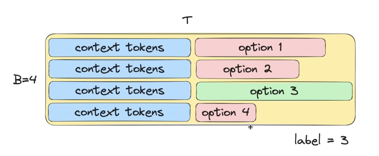
Using the above diagram as an illustration: we will take a batch size of 4, and tokenize each of the answer choices (the gaps indicate padded tokens, because the answer choices will have varying lengths). How do we get the language model to predict the most likely option? We can't get it to directly output the answer choice (for the above reason). So we will look at the probabilities for the tokens in the answer portion of each batch element. The answer choice with the highest probability of its answer tokens will tell us that the language model thinks this is the most likely answer choice.
Let's incorporate this HellaSwag eval into the main training script. First let's make torch.compile optional (it is interfering with the generation code and the eval code). Let's add a log file to track the train loss, val loss, HellaSwag accuracies. Every 250th iteration or last step we will evaluate with our validation loss. Every 250th iteration or last step we will evaluate with HellaSwag. Every 250th iteration or last step we will sample from our model (to judge qualitatively how our model is doing).
After 19073 iterations of 2**19 tokens (for a total of 10B tokens), here are some of the training and validation losses we get, as well as HellaSwag eval accuracy and sample outputs from the language model:
step 19066 | loss: 3.101273 | lr 6.0000e-05 | norm: 0.3020 | dt: 1712.10ms | tok/sec: 306225.48
step 19067 | loss: 3.045865 | lr 6.0000e-05 | norm: 0.3189 | dt: 1710.50ms | tok/sec: 306511.08
step 19068 | loss: 3.076556 | lr 6.0000e-05 | norm: 0.3206 | dt: 1709.35ms | tok/sec: 306717.35
step 19069 | loss: 3.092324 | lr 6.0000e-05 | norm: 0.2954 | dt: 1710.30ms | tok/sec: 306547.05
step 19070 | loss: 3.006369 | lr 6.0000e-05 | norm: 0.3059 | dt: 1713.07ms | tok/sec: 306050.96
step 19071 | loss: 2.994840 | lr 6.0000e-05 | norm: 0.3103 | dt: 1708.27ms | tok/sec: 306911.06
validation loss: 3.0732
HellaSwag accuracy: 3029/10042=0.3016
rank 0 sample 0: Hello, I'm a language model, and I am a computer science. This seems hard to me. Is it any wonder then that so few of us actually
rank 0 sample 1: Hello, I'm a language model, so am I?
And so... I think some parts of your world would be more suitable to teach than others.
rank 0 sample 2: Hello, I'm a language model, so I like that if your system does not look like a word in your dictionary, it is not a word.
rank 0 sample 3: Hello, I'm a language model, and what I'm doing is to model how speech is actually heard. In order to do that I start by thinking ahead
rank 1 sample 0: Hello, I'm a language model, and so I'm learning a lot while learning other languages. A lot of you are using Microsoft?
The video below
rank 1 sample 1: Hello, I'm a language model, a computer scientist and a computer nerd. I'm always open to new ideas and things, but mostly, I'm a
rank 1 sample 2: Hello, I'm a language model, I hate that you're asking me to do that. So yeah I have to do that. That's the first step
rank 1 sample 3: Hello, I'm a language model, and I'm really curious I'd like to know what sort of sentences it gives me here.
I'm trying to
step 19072 | loss: 3.108533 | lr 6.0000e-05 | norm: 0.3234 | dt: 38693.24ms | tok/sec: 13549.86
(venv) oagrawal@mew2:/nfs/oagrawal/andrej_2/build-nanogpt$

Min Train Loss: 2.882225
Min Validation Loss: 3.0732
Max Hellaswag eval: 0.3017
Sample outputs show coherent (if sometimes odd) completions. The entire pretraining run takes roughly 4 hours on 4 A100s.
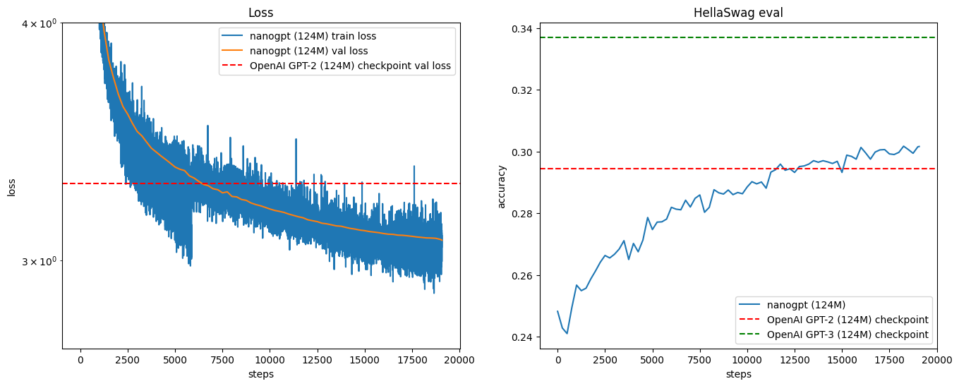
After 19073 × 3 = 57,219 iterations of 219 tokens (for a total of ~30B tokens), here are some of the training and validation losses we get, as well as HellaSwag eval accuracy and sample outputs from the language model:
step 57204 | loss: 2.963480 | lr 6.0000e-05 | norm: 0.5767 | dt: 871.15ms | tok/sec: 601832.53
step 57205 | loss: 2.997211 | lr 6.0000e-05 | norm: 0.5838 | dt: 871.94ms | tok/sec: 601287.34
step 57206 | loss: 2.974435 | lr 6.0000e-05 | norm: 0.5490 | dt: 874.14ms | tok/sec: 599774.78
step 57207 | loss: 2.956100 | lr 6.0000e-05 | norm: 0.5608 | dt: 872.37ms | tok/sec: 600991.71
step 57208 | loss: 2.999264 | lr 6.0000e-05 | norm: 0.5672 | dt: 872.11ms | tok/sec: 601168.66
step 57209 | loss: 2.974712 | lr 6.0000e-05 | norm: 0.7113 | dt: 873.83ms | tok/sec: 599991.45
step 57210 | loss: 3.003346 | lr 6.0000e-05 | norm: 0.5930 | dt: 873.00ms | tok/sec: 600560.70
step 57211 | loss: 2.870562 | lr 6.0000e-05 | norm: 0.5637 | dt: 875.02ms | tok/sec: 599171.43
step 57212 | loss: 2.954587 | lr 6.0000e-05 | norm: 0.7016 | dt: 872.06ms | tok/sec: 601206.95
step 57213 | loss: 2.954141 | lr 6.0000e-05 | norm: 0.6494 | dt: 872.27ms | tok/sec: 601064.81
step 57214 | loss: 2.966002 | lr 6.0000e-05 | norm: 0.6030 | dt: 873.81ms | tok/sec: 600002.91
step 57215 | loss: 2.953562 | lr 6.0000e-05 | norm: 0.5414 | dt: 872.39ms | tok/sec: 600976.93
step 57216 | loss: 2.923900 | lr 6.0000e-05 | norm: 0.5394 | dt: 871.67ms | tok/sec: 601472.53
step 57217 | loss: 2.838975 | lr 6.0000e-05 | norm: 0.5862 | dt: 873.05ms | tok/sec: 600527.57
validation loss: 2.9606
HellaSwag accuracy: 3281/10042=0.3267
rank 2 sample 0: Hello, I'm a language model, of course, if you need a word processor. If it doesn't exist yet, you can still use them. You
rank 2 sample 1: Hello, I'm a language model, the language model that I'm going to translate into KODO for today. So, you know, let's see
rank 2 sample 2: Hello, I'm a language model, so I don't need to have you define my model. You have this in mind. I mean, it's pretty
rank 2 sample 3: Hello, I'm a language model, I use syntax to implement the language model and how are I building a language model, how we look for patterns and ways
rank 3 sample 0: Hello, I'm a language model, and I'm not interested at all in using a class as a model, no matter what languages I create, how easy
rank 3 sample 1: Hello, I'm a language model, and it has a lot of variables, but it's just a bunch of variables.
So the question is is that
rank 3 sample 2: Hello, I'm a language model, and you've tried what you call a module by heart, but it doesn't work. How cool is that it was
rank 3 sample 3: Hello, I'm a language model, and most of them are right in the middle. So the languages you should be practicing right now are. I have a
rank 1 sample 0: Hello, I'm a language model, just an author. I write programs: a code is a computer program. How do I do things? Well, I
rank 1 sample 1: Hello, I'm a language model, you're going to be a real big star. What makes this programming language a language, you write a program and you
rank 1 sample 2: Hello, I'm a language model, I talk in C++, and I'm a system model with the same compiler. I can talk about a single byte
rank 1 sample 3: Hello, I'm a language model, and I'm using the GOTO button - I'm setting up a variable between the three operations that I'm going to
rank 0 sample 0: Hello, I'm a language model, and I use a lot of programming languages out there. Languages like SQL, and I have a friend, who is just
rank 0 sample 1: Hello, I'm a language model, so why do I care? Why should I bother. Language model is usually an important thing because language learning is a lot
rank 0 sample 2: Hello, I'm a language model, so I will ask you question. If you do, please leave the questions in the comment section.
I am always
rank 0 sample 3: Hello, I'm a language model, not a teacher. I'm not a linguist, but I still like the learning that occurs when I learn new phrases
step 57218 | loss: 2.878605 | lr 6.0000e-05 | norm: 0.5963 | dt: 21803.57ms | tok/sec: 24045.97
Sample outputs are much more coherent now.
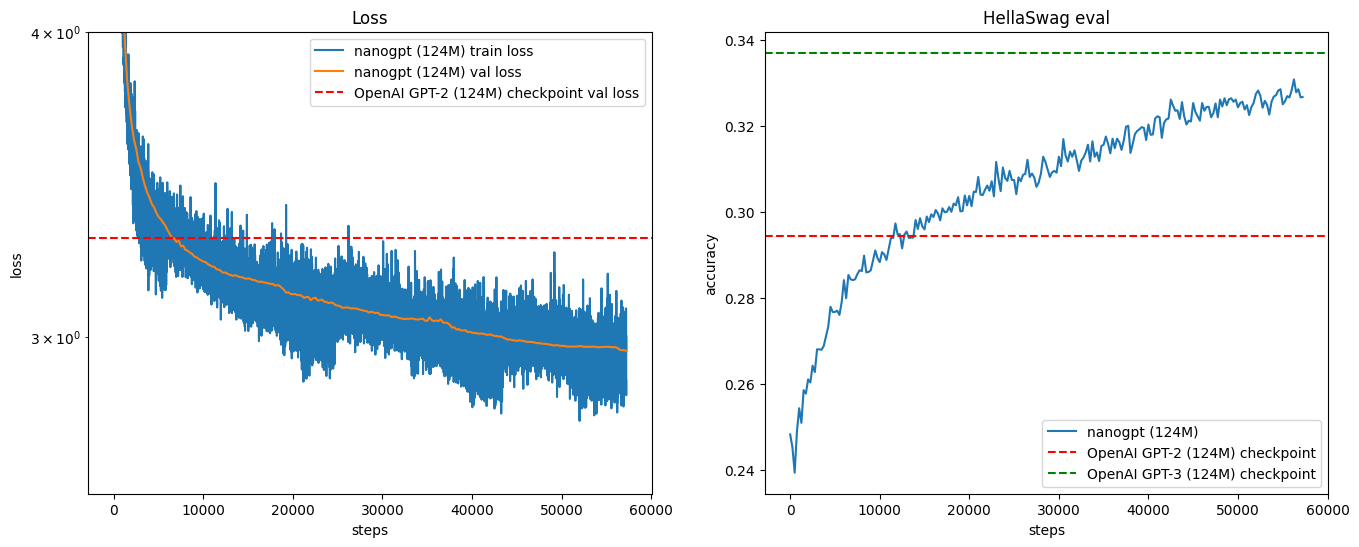
Summary
Summary of all we've gone through: We were looking at the GPT 2 and GPT 3 papers. We learned how to set up these training runs. We wrote all the classes from scratch (e.g. CausalSelfAttention, etc.). We looked at the training and val losses, and the HellaSwag eval, and compared performance between our model and GPT 2 and GPT 3 performance. Thanks a lot to Andrej Karpathy!