In this lecture, we will go back and forth between a VS Code codebase, where we will incrementally build a character-level language model using transformers, and a Google Colab notebook, which we will use to explain the results. This lecture is inspired by the paper Attention is All You Need, which introduced the transformer architecture. We are going to train a transformer-based, character-level language model. Instead of training on the entire internet, we will use the Tiny Shakespeare dataset.
Tokenizer + Train / Val Split
First, we download the Tiny Shakespeare dataset. Then, we identify all the unique characters in the dataset and sort them. The ordering is arbitrary, and we find that there are 65 unique characters. We then create an encoder and a decoder. The encoder maps each character to an integer representation (from 0 to 64), and the decoder maps the integer back to the character. Using this simple encoder, we can now encode the entire Tiny Shakespeare dataset into a sequence of integers.
We will use the first 90% of the data as our training set and the remaining 10% as our validation set. The validation set helps us determine if our model is overfitting. Overfitting occurs when the model performs very well on the data it was trained on but fails to generalize to new, unseen data. Since we want our language model to not only reproduce the training data but also to improvise and generate novel text from a random starting point, it's crucial to monitor and prevent overfitting.
Data Loader
Feeding the entire dataset to the transformer at once for training is computationally inefficient. Instead, we feed it smaller "blocks" of data. For example, consider the first 9 characters of our dataset, represented as the tensor tensor([18, 47, 56, 57, 58, 1, 15, 47, 58]). From this single chunk, we can derive multiple training examples. If you feed the model the character `18`, it should predict `47`. If you feed it `18` and `47`, it should predict `57`, and so on.
When input is tensor([18]) the target: 47
When input is tensor([18, 47]) the target: 56
When input is tensor([18, 47, 56]) the target: 57
When input is tensor([18, 47, 56, 57]) the target: 58
When input is tensor([18, 47, 56, 57, 58]) the target: 1
When input is tensor([18, 47, 56, 57, 58, 1]) the target: 15
When input is tensor([18, 47, 56, 57, 58, 1, 15]) the target: 47
When input is tensor([18, 47, 56, 57, 58, 1, 15, 47]) the target: 58
Here are the 8 examples hidden in a chunk of 9 characters. Note: we do this "nested" example method not just for efficiency reasons (e.g., because we already have the next tokens so why not). There is also some theoretical advantage to this - this will make our model be able to predict the next token with as little as one token of context and as much as block size tokens of context. After we have block size amount of tokens we will need to start truncating the context amount.
We've looked at the time dimension now. There is another dimension to think about - the batch dimension. Instead of just processing one chunk at a time, we would like to process multiple chunks at a time. This is done because GPUs are very good at parallel processing - if we don't do this then it's essentially wasting compute that could have been used.
Start with Modeling - Simplest Neural Network: Bigram Language Model
We'll begin with the simplest possible neural network: a Bigram Language Model. In this model, the prediction of the next character is based solely on the current character. The forward pass consists of looking up the current character in an embedding table to get the logits for the next character. To evaluate the model's performance, we'll use the negative log-likelihood loss function, which is implemented as `F.cross_entropy()` in PyTorch. We can also use this model to generate text, though initially, the output will be random because the model's weights are initialized randomly. Let's train this network using the Adam optimizer, which is an alternative to the Stochastic Gradient Descent (SGD) we've used in previous posts.
Here is the code for this:
import torch
import torch.nn as nn
from torch.nn import functional as F
torch.manual_seed(1337)

class BigramLanguageModel(nn.Module):
    def __init__(self, vocab_size):
        super().__init__()
        # each token directly reads off the logits for the next token from a lookup table
        self.token_embedding_table = nn.Embedding(vocab_size, vocab_size)

    def forward(self, idx, targets=None):
        # idx and targets are both (B,T) tensor of integers
        logits = self.token_embedding_table(idx)  # (B,T,C)
        if targets is None:
            loss = None
        else:
            B, T, C = logits.shape
            logits = logits.view(B*T, C)
            targets = targets.view(B*T)
            loss = F.cross_entropy(logits, targets)
        return logits, loss

    def generate(self, idx, max_new_tokens):
        # idx is (B, T) array of indices in the current context
        for _ in range(max_new_tokens):
            logits, loss = self(idx)
            logits = logits[:, -1, :]  # becomes (B, C)
            probs = F.softmax(logits, dim=-1)  # (B, C)
            idx_next = torch.multinomial(probs, num_samples=1)  # (B, 1)
            idx = torch.cat((idx, idx_next), dim=1)  # (B, T+1)
        return idx

m = BigramLanguageModel(vocab_size)
logits, loss = m(xb, yb)
print(logits.shape)
print(loss)

idx = torch.zeros((1, 1), dtype=torch.long)
print(decode(m.generate(idx, max_new_tokens=100)[0].tolist()))
Output for random weights:
torch.Size([32, 65])
tensor(4.8786, grad_fn=)

SKIcLT;AcELMoTbvZv C?nq-QE33:CJqkOKH-q;:la!oiywkHjgChzbQ?u!3bLIgwevmyFJGUGp
wnYWmnxKWWev-tDqXErVKLgJ
optimizer = torch.optim.AdamW(m.parameters(), lr=1e-3)
batch_size = 32
for steps in range(20000): # increase number of steps for good results...
xb, yb = get_batch('train')
logits, loss = m(xb, yb)
optimizer.zero_grad(set_to_none=True)
loss.backward()
optimizer.step()
print(loss.item())
# output: 2.576992988586426
print(decode(m.generate(idx, max_new_tokens=400)[0].tolist()))Output after training:
IUS: plllyss,
BOricand t me kusotenthayorieanatin inou idis ne horsercoownd
ORGunde ll mugl wrg g be, to fr t athame-he's h f we frs it tepodestha wird ad s; belesuin byes mb. Ond tand m:
Wed toshoths 'd ath! s pouthas COPrgoomur d y; withefeloulorneey mya chile.
SThyof wiorimy heig, ond watomow b,
CKitounghat Isouce t gfonyome,
FFoul hacyerrabayo
As censtharyoty, myof n, moo doy Bofofoye athar bu
Reasonable, ish....
Almost Ready for Transformers
Our bigram model has a significant limitation: it only uses one preceding character to predict the next one. To build a more powerful model, we want to incorporate information from all previous tokens in the sequence. For a token at position `t`, the model should consider tokens at positions `t`, `t-1`, and so on, all the way back to the beginning. A simple way to achieve this is to average the embeddings of all tokens up to and including the current position `t`.
Here is how you can implement this (consider the following toy example):
torch.manual_seed(1337)
B, T, C = 4, 8, 2  # batch, time, channels
x = torch.randn(B, T, C)
# We want x[b,t] = mean_{i<=t} x[b,i]
xbow = torch.zeros((B, T, C))
for b in range(B):
    for t in range(T):
        xprev = x[b, :t+1]  # (t, C)
        xbow[b, t] = torch.mean(xprev, 0)
Now if we look at the first batch and the averaged version of this, we see that the first element (first row) is the same as the first input row, but the second element is the average of the first two rows, etc. This is called a "bag of words."
We have two for loops - this is pretty inefficient. How can we make this more efficient? With matrix multiplication!
So, what are we trying to accomplish? For a single batch element, we have a tensor of size `T x C` (time x channels). We want to produce an output tensor where the first row is identical to the first row of the input, the second row is the column-wise average of the first two input rows, the third row is the average of the first three input rows, and so on. Can we achieve this with a matrix multiplication? Yes, we can construct a `T x T` matrix to perform this operation. The first row of this matrix would be `[1, 0, 0, ...]`, which, when multiplied, selects the first input row. The second row would be `[0.5, 0.5, 0, 0, ...]`, which averages the first two input rows. Continuing this pattern reveals that the required `T x T` matrix is a lower triangular matrix. We can create it with the following code:
a = torch.tril(torch.ones(T, T))
a = a / torch.sum(a, 1, keepdim=True)
So instead of the for loop version, we can do:
wei = torch.tril(torch.ones(T, T))
wei = wei / wei.sum(1, keepdim=True)
xbow2 = wei @ x  # (B, T, T) @ (B, T, C) -> (B, T, C)
# Torch broadcasting rules will make the extra dimension of B for the wei tensor, and independently apply the T x T matrix on the T x C matrix, to get exactly the result we want!
Now we can write the above commands in yet another manner:
tril = torch.tril(torch.ones(T, T))
wei = torch.zeros((T, T))
wei = wei.masked_fill(tril == 0, float('-inf'))
wei = F.softmax(wei, dim=-1)
xbow3 = wei @ x
Why do we want this third version if it is doing the same thing? Because of this crucial line: wei = torch.zeros((T, T)). For now we are setting these to be zero, saying that all previous tokens are equally important for all tokens, but as soon as we begin transformers these weights will not be constant. Some words will find certain other words more or less interesting. Some words will pay more or less "Attention" to these words.
We will now build upon our bigram model. Instead of mapping an input token embedding directly to an output prediction, we will introduce a layer of indirection. We'll still use an embedding table, but its dimension will be independent of the vocabulary size. The output of this embedding will then be fed into a linear layer that projects it to the vocabulary size dimension.
We also want to incorporate positional information for each character. To do this, we'll create a `position_embedding_table`. In the forward pass, we'll generate positional indices using torch.arange(T, device=device) and look up their embeddings. This gives us a `T x C` tensor of positional embeddings, which we add to the token embeddings. This way, the model receives information not only about what the tokens are but also where they are in the sequence. While this positional information doesn't significantly help our simple bigram model, it will become crucial when we introduce self-attention, as it will allow tokens to communicate with each other effectively.
OKAY NOW LET'S IMPLEMENT SELF ATTENTION!!!
Back to the trick in self.attention - we have the following piece of code:
torch.manual_seed(1337)
B, T, C = 4, 8, 32  # batch, time, channels
x = torch.randn(B, T, C)

tril = torch.tril(torch.ones(T, T))
wei = torch.zeros((T, T))
wei = wei.masked_fill(tril == 0, float('-inf'))
wei = F.softmax(wei, dim=-1)
out = wei @ x
Previously, our `wei` matrix started with all zeros, which was then normalized to give equal attention (affinity) to all previous tokens. We want to make this data-dependent, allowing a token to decide how much attention it pays to other tokens. Self-attention achieves this by having each token emit two vectors: a **query** and a **key**. The query vector represents "what am I looking for?" and the key vector represents "what do I contain?". The affinity between tokens is then calculated by taking the dot product of their query and key vectors.
Let's implement a single "head" of self-attention. The `head_size` is a hyperparameter. The key and query vectors are generated through linear transformations (matrix multiplications without a bias term) of the input.
head_size = 16
key = nn.Linear(C, head_size, bias=False)
query = nn.Linear(C, head_size, bias=False)

k = key(x)    # (B, T, C) -> (B, T, 16)
q = query(x)  # (B, T, C) -> (B, T, 16)

wei = q @ k.transpose(-2, -1)  # (B, T, 16) @ (B, 16, T) -> (B, T, T)
So now instead of the all 0s for wei (indicating equal affinity to all previous tokens), we can use this data dependent affinity matrix.
One more crucial detail: we don't use the `wei` affinities to aggregate the raw token embeddings directly. Instead, we aggregate **value** vectors. Each token also produces a value vector, which is generated in the same way as the key and query vectors (through a linear transformation).
value = nn.Linear(C, head_size, bias=False)
v = value(x)  # B T C -> B T head_size
out = wei @ v  # B T T @ B T head_size => B T head_size
out.shape  # torch.Size([4, 8, 16])
You can think of raw token embedding as private info about tokens - so the queries are "what am I looking for?", keys are "what information I contain", and value is "if you find me interesting, here is what I will communicate to you."
Notes About Self-Attention
Attention can be thought of as a communication mechanism over a directed graph. In our case, with a sequence length of 8, we have a graph of 8 nodes. The first node points to itself; the second node is pointed to by the first two nodes, and so on, up to the eighth node.
A key property of this mechanism is that the nodes have no inherent sense of their position in space. This is why we need positional encodings. This contrasts with convolutional layers, which are explicitly designed to operate over a spatial grid.
Within a batch, items are processed independently. In our graph analogy, a batch size of 4 means we are processing four separate, parallel directed graphs.
The type of attention we are implementing is for autoregressive language modeling (i.e., text generation), where a token can only attend to past tokens. However, this isn't always the case. For tasks like sentiment analysis, a token might attend to future tokens as well.
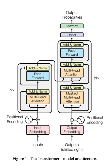
What we are building is known as a "decoder block." It's called a decoder because its autoregressive structure is used to "decode" an answer or generate a sequence. The "self" in self-attention comes from the fact that the keys, queries, and values all originate from the same input source, `x`. Attention is a more general concept; in "cross-attention," for example, queries might come from one source while keys and values come from another, allowing different parts of a model (like an encoder and decoder) to communicate.
A final implementation detail from the Attention is All You Need paper is scaled attention. The affinity matrix (`wei`) is divided by the square root of the `head_size`. This scaling factor is important for stabilizing training. Without it, the dot product of the key and query vectors can grow large, pushing the softmax function into regions with very small gradients.
Now Let's Change Our Codebase With This Self Attention Block
We will add one Attention Head to this codebase:
class Head(nn.Module):
    """one head of self-attention"""
    def __init__(self, head_size):
        super().__init__()
        self.key = nn.Linear(n_embd, head_size, bias=False)
        self.query = nn.Linear(n_embd, head_size, bias=False)
        self.value = nn.Linear(n_embd, head_size, bias=False)
        self.register_buffer('tril', torch.tril(torch.ones(block_size, block_size)))

    def forward(self, x):
        B, T, C = x.shape
        k = self.key(x)
        q = self.query(x)
        wei = q @ k.transpose(-2, -1) * C**-0.5  # (B, T, C) @ (B, C, T) -> (B, T, T)
        wei = wei.masked_fill(self.tril[:T, :T] == 0, float('-inf'))
        wei = F.softmax(wei, dim=-1)
        v = self.value(x)
        out = wei @ v
        return out
This should look very familiar given our attention experiments in Google Colab. Now to embed this attention head into the existing language model, after the token embeddings and position embeddings are added together and before passing to the linear layer that gets us to our logits, we send it through the self.attention block - note that we are passing in n_embd as our head_size, so if you input a (B, T, C) tensor we will also get a (B, T, C) tensor - this way we can straight away pass the output of the attention block to the linear layer.
Let's keep working - our model is far from perfect right now. If you look into the Attention is All You Need paper, there is something called multi-head attention. What is multi-head attention? Instead of a single head of attention, you get multiple heads of attention in parallel, concat the result all together. See the diagram from the paper below:
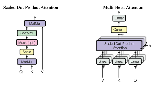
Let's apply this to our codebase. One note: typically when we increase number of heads we also decrease the number of channels for each of these heads as well - here we went from a single attention head with 32 channels to 4 attention heads running in parallel each with 8 dimensions.
When we look at the self attention block from the paper, we see that there are some similarities between what we've implemented so far and what the paper describes - we have the token embeddings, the position embeddings, the multi head attention. But there are some differences as well - we don't have the multi head attention that combines information from the encoder to put in the decoder (that is for encoder-decoder architectures - we aren't building that here, we are trying to build a decoder-only network for text generation). Also we see that before the final linear layer that maps our embedding dimension to the vocab size, inside of each attention block after the multi head self attention block there is a feed forward block - we will implement this feed forward network.
Why do we need this feed forward network? What is the intuition behind this feed forward network? The intuition is the tokens have communicated amongst each other via the multi head self attention, but each token hasn't gotten enough time to think about the information it's received. Once we implement this into our codebase our validation loss drops even more (not by much but still an improvement).
Now we will intersperse the communication with the computation - instead of just having one attention block, let's repeat the attention block. So now we will have the first block's multi head attention then the first block's feed forward network, then the second block's multi head self attention then the second block's feed forward layer, etc.
Another change is residual connections - you may have seen from the transformer architecture that there are lines around the multi head self attention and the feed forward network in each block - these are residual connections!
For each block instead of having:
def forward(self, x):
    x = self.sa(x)
    x = self.ffwd(x)
    return x
You have:
def forward(self, x):
    x = x + self.sa(x)
    x = x + self.ffwd(x)
    return x
What difference does this make? Because we are doing addition here, when you do backpropagation, for the addition operator the gradient flows through both "branches" - by adding a residual connection for the multi head self attention and the feed forward for each block, we are essentially building a highway for the gradient to reach the input really fast. In fact in the beginning of training the gradient flows straight to the inputs, and only later do the gradients start affecting the multi head self attention blocks and the feedforward network.
Another note - because we are adding residual connections around the multihead self attention and feed forward layers, at the end of these modules we will add a projection. For the self attention this projection will be from n_embd to n_embd. For feed forward we will change things up a little: we add more compute - the FFN goes from n_embd to 4*n_embd (ReLU) to n_embd.
Layer Norm
Now we will implement another thing that will help with training - layer norm. Remember we implemented batch normalization before? Where we normalize across the batch dimension - to make each node have zero mean and unit std dev. What is the difference between BatchNorm and LayerNorm? Instead of normalizing across the batch dimension - we normalize across rows - in other words it normalizes each example rather than across examples in a batch. Another note - from the transformer diagram they normalized after the transformation - since then people have figured out to normalize before the transformation. When we do layer norm, we will normalize across the channel dimension (the batch and time dimensions act like batch dimensions).
Scaling Up
At this point we have a pretty solid transformer network - let's try to scale this up. We added dropout layers - we add this at the very end of multi head self attention and feed forward (right before we are merging the residual path with the residual connection) and we can also drop out before we use wei to compute our affinities right before we dot product with the values - this is like randomly preventing some tokens from talking to each other - we add it here as a regularization technique so that we can prevent overfitting as we scale up.
Here are the hyperparameters: batch_size=64, block_size=256, max_iters=5000, eval_interval=500, learning_rate=3e-4, device='cuda' if torch.cuda.is_available() else 'cpu', eval_iters=200, n_embd=384, n_head=6 (so each block in our multi head attention will have 64 channels), n_layer=6 (we have 6 blocks stacked on top of each other), dropout=0.2 (20 percent of neurons will be deactivated each forward and backward pass randomly).
Not too bad! Why does the Attention is All You Need look a little different than what we built? They were dealing with machine translation (e.g., French to English). They would take French and pass it to an encoder block, then the decoder blocks start decoding English, conditioned on the French. This mixture happens in the second multi head attention (instead of self attention though it is cross attention here).
How Can We Train ChatGPT Ourselves?
So, how could we train a model like ChatGPT ourselves, based on what we've learned? The process involves two main stages: **Pre-training** and **Fine-tuning**.
The pre-training phase is what we've just done. We feed massive amounts of text into a decoder-only transformer block and train it to predict the next token. This results in a model that is good at completing documents-essentially, a very sophisticated "babbler." The primary difference between our model and something like GPT-3 lies in the scale. We trained a 10 million parameter model on about 300,000 tokens on a single GPU. GPT-3 has 175 billion parameters and was trained on 300 billion tokens. Architecturally, the models are very similar, but the sheer scale of the data, model size, and computational resources required for GPT-3 presents immense infrastructure challenges.
After pre-training, the model is a document completer, not a conversational chatbot. To create a chatbot and align it with human preferences, a three-stage fine-tuning process is used. First, the model is fine-tuned on a dataset of question-and-answer examples. Second, human labelers rank different model responses to the same prompt, and this ranking data is used to train a separate "reward model." Finally, this reward model is used to further fine-tune the language model using a reinforcement learning algorithm called Proximal Policy Optimization (PPO). This entire fine-tuning stage is crucial for creating a helpful and harmless AI assistant.
Thanks a lot to Andrej Karpathy!