Om Agrawal

Intro

As we think about making larger models, we need to look into some key aspects of our models: the activations and the gradients. By studying activations and gradients we will learn that currently we are handling our activations and gradients very haphazardly. To train deeper neural networks reliably, we will need a mechanism that will stabilize the activations - the mechanism I am talking about is BatchNorm layer. Additionally, studying activations during training and gradients during backprop will help us understand the history of the later models -> RNNs, GRUs, Transformers, etc while RNNs are universal approimators, not easily optimizable with first order gradient techniques that we use. why are they not optimazable? key is to understand gradients and activations and how they behave during trainnig. GRUs and Transformers have tried to improve that situation.

Here is our model so far:

words = open('names.txt', 'r').read().splitlines()

chars = sorted(list(set(''.join(words))))
stoi = {s:i+1 for i,s in enumerate(chars)}
stoi['.'] = 0
itos = {i:s for s,i in stoi.items()}
vocab_size = len(itos)

block_size = 3 # context length: how many characters do we take to predict the next one?

def build_dataset(words):  
  X, Y = [], []
  
  for w in words:
    context = [0] * block_size
    for ch in w + '.':
      ix = stoi[ch]
      X.append(context)
      Y.append(ix)
      context = context[1:] + [ix] # crop and append

  X = torch.tensor(X)
  Y = torch.tensor(Y)
  print(X.shape, Y.shape)
  return X, Y

import random
random.seed(42)
random.shuffle(words)
n1 = int(0.8*len(words))
n2 = int(0.9*len(words))

Xtr,  Ytr  = build_dataset(words[:n1])     # 80%
Xdev, Ydev = build_dataset(words[n1:n2])   # 10%
Xte,  Yte  = build_dataset(words[n2:])     # 10%

n_embd = 10 # the dimensionality of the character embedding vectors
n_hidden = 200 # the number of neurons in the hidden layer of the MLP

g = torch.Generator().manual_seed(2147483647) # for reproducibility
C  = torch.randn((vocab_size, n_embd),            generator=g)
W1 = torch.randn((n_embd * block_size, n_hidden), generator=g) 
b1 = torch.randn(n_hidden,                        generator=g)
W2 = torch.randn((n_hidden, vocab_size),          generator=g) 
b2 = torch.randn(vocab_size,                      generator=g) 

parameters = [C, W1, b1, W2, b2]
for p in parameters:
  p.requires_grad = True

max_steps = 200000
batch_size = 32
lossi = []

for i in range(max_steps):
  
  # minibatch construct
  ix = torch.randint(0, Xtr.shape[0], (batch_size,), generator=g)
  Xb, Yb = Xtr[ix], Ytr[ix] # batch X,Y
  
  # forward pass
  emb = C[Xb] # embed the characters into vectors
  embcat = emb.view(emb.shape[0], -1) # concatenate the vectors
  # Linear layer

  # insight in batch normalization paper, just normalize them!
  hpreact = embcat @ W1 + b1 # hidden layer pre-activation
    
  # Non-linearity
  h = torch.tanh(hpreact) # hidden layer
  logits = h @ W2 + b2 # output layer
  loss = F.cross_entropy(logits, Yb) # loss function
  
  # backward pass
  for p in parameters:
    p.grad = None
  loss.backward()
  
  # update
  lr = 0.1 if i < 100000 else 0.01 # step learning rate decay
  for p in parameters:
    p.data += -lr * p.grad
            

Here are our losses:

train 2.1282482147216797
val 2.1710422039031982
                

Let’s try to improve our model, and in that process demonstrate why BatchNorm would be useful.

First thing is first, the initial loss is too high. Even if we had a completely uniform distribution for the prediction of the next character, that means the loss would be:

-torch.tensor(1/27.0).log()
# tensor(3.2958)
            

So we want the logits to be 0, or roughly equal. We are getting the logits by doing:

logits = h @ W2 + b2 # output layer
            

To make the logits 0, we can try to make b2 zero, and W2 close to 0 (dont change the h, as those are values calculated from the previous layers). We make the following changes:

W2 = torch.randn((n_hidden, vocab_size),          generator=g) * 0.01 # make logits initally be close to 0
b2 = torch.randn(vocab_size,                      generator=g) * 0 # make logits at init be close to 0
            

after decreasing b2 and W2, losses are:

train 2.069589138031006
val 2.1310746669769287
            

Okay, logits are okay, but this is like cleaning the outside of the cage without taking care of the bird inside. Let’s look deeper - there is a deeper problem with the activations of the hidden layer.

h.shape:

torch.Size([32, 200])
            

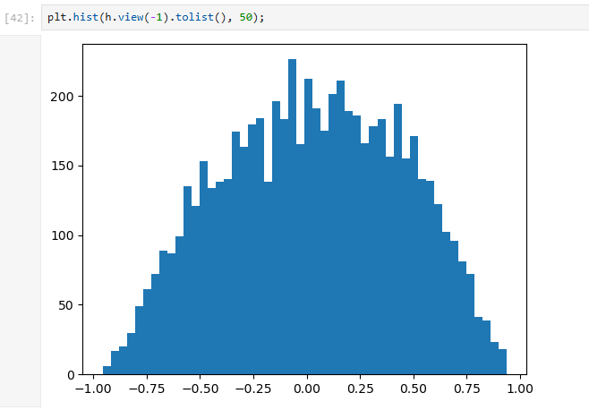
plt.hist(h.view(-1).tolist(), 50);

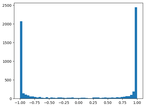
Most values are -1 and 1, tanh is very active.

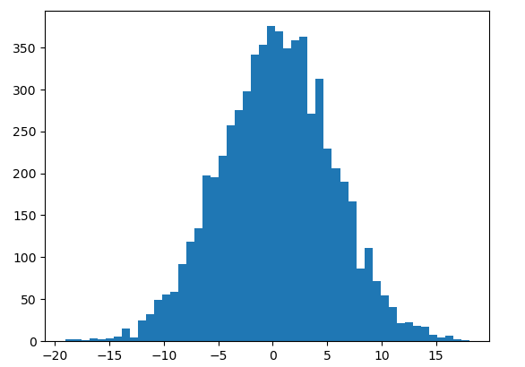
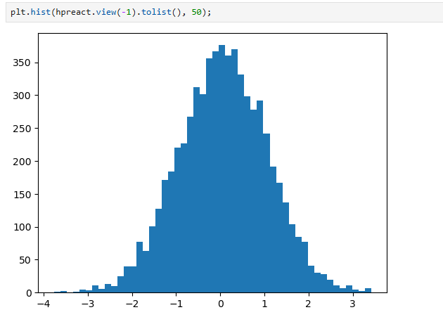
Why is this? Because the preactivation distribution is very broad:

plt.hist(hpreact.view(-1).tolist(), 50);

Why are the activations being so a problem? Lets look at the micrograd code we had written:

def tanh(self):
    x = self.data
    t = (math.exp(2 * x) - 1) / (math.exp(2 * x) + 1)
    out = Value(t, (self,), 'tanh')
    def _backward():
        self.grad += (1 - t ** 2) * out.grad
    out._backward = _backward
    return out
            

When the outputs of the preactivation are 1 or -1, then we set self.grad = (1 - t*2) * out.grad, whatever out.grad was, we are killing the backprop because our t value is 1 or -1. When tanh is 0, the tanh unit is inactive and the gradient passes through. The closer you are to 1 or -1, the more the grad is squashed. If all of these outputs of h (after the tanh) are 1 or -1, the gradients that are flowing through tanh are stopped

Essentially, if the activations for a tanh neuron are 1 or -1, we kill the gradients, and no learning happens.

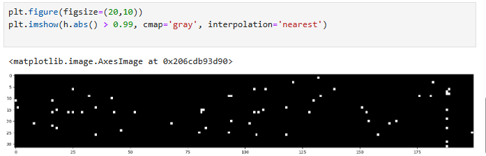
Let's see the health of the h layer (after tanh):

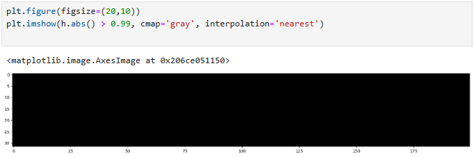
plt.figure(figsize=(20,10))

plt.imshow(h.abs() > 0.99, cmap='gray', interpolation='nearest')

The image below has a shape of 32 * 200, as it's 200 neurons (on the x-axis), for the 32 examples (y-axis)

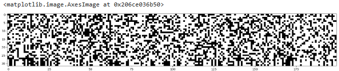
A lot of the image is white, which means the tanh neurons are very “active”. This means that they are all are in the flat tail of the tanh function, where their gradient is being destroyed. Thank goodness we dont see a white column. If an entire column were white, that would mean we have a dead neuron, where no single example activates it in the non-flat region, and it will never learn. At least neurons are learning from some example, but you can see how this is not an ideal scenario.

BTW, this is not just an issue for tanh non-linearities. The sigmoid non-linearity also has this issue, and so does ReLU (for values less than 0). Leaky ReLU and ELU suffer less from this. A neuron can become overactivated at initialization of the weights and biases (like it occurred for us), but also if the learning rate is too high. A high learning rate can knock a neuron out of the data manifold, and the neuron can remain dead forever. This is like "brain damage" in the mind of a neural network.

W1 = torch.randn((n_embd * block_size, n_hidden), generator=g) * 0.1
b1 = torch.randn(n_hidden,                        generator=g) * 0.01
                

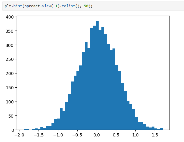
The hpreact distribution is now better:

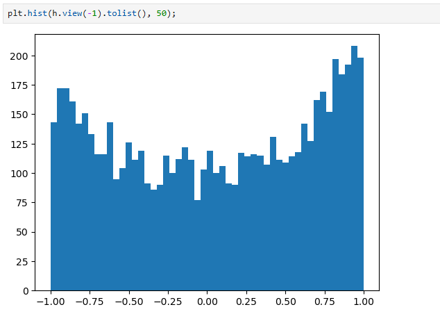
The h distribution (after tanh) is also better:

When we look at the health of the neural net, here’s what we see:

Maybe we should have a few white neurons…

W1 = torch.randn((n_embd * block_size, n_hidden), generator=g) * 0.2
b1 = torch.randn(n_hidden,                        generator=g) * 0.01
            

After fixing tanh saturation, our losses are:

train 2.0355966091156006
val 2.1026785373687744
            

How do you come up with magic numbers like 0.2? How do you set this when you have a neural network with lots and lots of layers?

Kaiming init:

g = torch.Generator().manual_seed(2147483647) # for reproducibility
C  = torch.randn((vocab_size, n_embd),            generator=g)
W1 = torch.randn((n_embd * block_size, n_hidden), generator=g) * 0.2
b1 = torch.randn(n_hidden,                        generator=g) * 0.01
W2 = torch.randn((n_hidden, vocab_size),          generator=g) * 0.01 # make logits initally be close to 0
b2 = torch.randn(vocab_size,                      generator=g) * 0 # make logits at init be close to 0
            

Turns out there are principled ways of settings these scales.

Take this case for example:

x = torch.randn(1000, 10)
w = torch.randn(10, 200) 
y = x @ w
            

x and w by themselves have a gaussian distribution, but when you get their dot product, you find that the spread of the dot product's distribution is larger. In Neural Networks, we don't want our preactivations to explode (and you can see how this problem can be made worse as we increase the number of layers). How do we keep the preactivations from expanding?

Well we can element-wise divide the w matrix by some scalar. But by how much? We are back at our original question: how do we set these scalars in principled ways?

From here, we learn that if we want to preserve the spread of the dot product, we divide by the square root of the number of input elements.

x = torch.randn(1000, 10)
w = torch.randn(10, 200)  / 10**0.5 # divide by sqrt of fanin (number of inputs)
y = x @ w
            

The spread of y here is exactly 1 (just like the spread of x and w). How do we do something similar in the presence of multiple layers in a neural network with nonlinearities?

There is a research paper that looks into this: Delving Deep into Rectifiers: Surpassing Human-Level Performance on ImageNet Classification.

From this paper, because they used the ReLU non-linearity, they found that they needed to keep the standard deviation at sqrt(2/fan_in). Again, fan_in is the number of input features. So how do you make the gaussian have a certain standard deviation?

If you do torch.randn(10000), you have 10,000 numbers that form a gaussian distribution (mean 0, std dev 1). If we want to make the std dev be a certain number, say x, then all we need to do is element-wise multiply all the values by x.

So if we want the values in our weight matrix to have a standard deviation of sqrt(2/fan_in), all we need to do is multiply by sqrt(2/fan_in).

Now, we are going with sqrt(2/fan_in) because the paper used the ReLU non-linearity. But for a general non-linearity, we want to set the std dev to be gain / sqrt(fan_in). The value of the gain depends on which non-linearity you are using.

The paper not only shows how to keep the std dev of the activations in the forward pass stable, but it also studies how to keep the distribution of gradients in the backward pass stable as well. They found that, if you keep one stable (say we keep activations in the forward pass stable by keeping the std dev gain / sqrt(fan_in)), the spread of the other will be okay too (so gradients will be okay too, no need to stabilize those separately.)

This initialization of the weights, which sets the standard deviation to gain / sqrt(fan_in), is called Kaiming initialization (Kaiming was the first author on the paper).

# how to init weights in pytorch?
# torch.nn.init.kaiming_normal_(tensor, a=0, mode='fan_in', nonlinearity='leaky_relu', generator=None)
# mode - normalize activations or gradients? paper says doesnt matter, keep it as default - 'fan-in'
# nonlinearity type - gain will be different
            

What does gain represent? Why do we need it? Tanh is a squashing function, so to fight the squeezing, we need to boost the values to normalize them.

A couple of years ago, the initialization of weights mattered a lot to keep the distribution of activations and gradients in check. But now, modern innovations keep everything more well-behaved and stable. Examples of these innovations include residual connections, normalization layers (batch normalization, layer normalization, group normalization), and better optimizers (not just SGD, but also Adam, RMSProp).

So, with all of these modern innovations, people often just divide the weight matrix element-wise by the square root of the fan-in. If we want to be more precise, we want to set the standard deviation to be gain / sqrt(fan_in).

After implementing Kaiming initialization for W1, here are our losses. Note they are not all that different, but this initialization strategy is crucial for neural networks much deeper than ours:

After Kaiming init for W1, we get roughly similar losses:

train 2.0376641750335693
val 2.106989622116089
            

BatchNorm Layer:

Here is the paper: Batch Normalization: Accelerating Deep Network Training by Reducing Internal Covariate Shift.

The BatchNorm Layer’s impact was that it made it possible to reliably train deep neural networks.

We have hidden states hpreact. We don't want them to be exactly 0, because if they are, then the “tanh” nonlinearity isn’t doing anything. But we also don't want to saturate the tanh (all values being 1 or -1), otherwise the neuron isn’t learning. We want a roughly gaussian distribution with a mean of 0 and a standard deviation of 1, at least at initialization. The insight from the paper is to take the hidden states and make them roughly gaussian by subtracting the mean and dividing by the standard deviation. This normalization is perfectly differentiable.

From the paper, here is the formula for batch normalization:

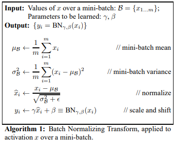
In code, we can implement this with:

hpreact = (hpreact - hpreact.mean(0, keepdims=True)) / hpreact.std(0, keepdims=True)
            

(Every single neuron will be unit gaussian on these 32 examples in the batch, normalizing these batches)

Okay, this is all well and good. We want the gaussian distribution at initialization, but we don't want the distribution to always be gaussian throughout training. Instead, we want the neural net to be able to move the preactivations around to be diffuse, sharp, or more/less trigger-happy. For this, in addition to normalizing, let's introduce a gain and bias to scale and offset the distribution.

In our small neural network, batch normalization will not do much. But when we have a much deeper neural network, it will become much harder to tune the weight matrices to make sure the preactivations are all roughly gaussian. Compared to that, it would become much easier to sprinkle these batch normalization layers throughout the neural network. In practice, when we have a linear layer or a convolutional layer, it is customary to append a batch normalization layer to control the scale of the activations at every point of the neural net. This controls the scale of the activations and means we don't need precise mathematics for other components in the neural net (e.g. the Kaiming init we introduced for W1). This significantly stabilizes training for deep neural networks.

However, there is a cost. Before batching, each logit was just a function of its input (and no other input in the batch). But now with batch normalization, the logits are not just a function of that input, but are also a function of all of the other examples in the batch. You would think this would be undesirable, but in a strange way, it helps the neural net not overfit, acting as a regularizer. This second-order effect makes it even better. Even if we want to try to create better alternatives to batch normalization, we are incentivized not to because of the first and second-order benefits of batch normalization.

There are several other things we need to deal with as a side effect of batch norm. For example, the fact that examples are grouped together in the forward and backward pass leads to strange side effects. How do we do inference for just one example? We need to calculate the batch norm mean and standard deviation one last time after training.

Here is the code for that:

# calibrate the batch norm at the end of training

with torch.no_grad():
  # pass the training set through
  emb = C[Xtr]
  embcat = emb.view(emb.shape[0], -1)
  hpreact = embcat @ W1 # + b1
  # measure the mean/std over the entire training set
  bnmean = hpreact.mean(0, keepdim=True)
  bnstd = hpreact.std(0, keepdim=True)
            

So at inference time we can use these calculated values:

hpreact = bngain * (hpreact - bnmean) / bnstd + bnbias
            

Even with this solution, no one wants to estimate this bnmean and bnbias as a second step of neural network training. No one wants to do a training loop, and then another loop for calculating the bnmean and bnstd! Instead, we can estimate this in a running manner. This will give us a rough estimation of the bnmean and bnstd.

Here is what the batch norm section of our forward pass looks like:

# BatchNorm layer
# -------------------------------------------------------------
bnmeani = hpreact.mean(0, keepdim=True)
bnstdi = hpreact.std(0, keepdim=True)
hpreact = bngain * (hpreact - bnmeani) / bnstdi + bnbias
with torch.no_grad():
    bnmean_running = 0.999 * bnmean_running + 0.001 * bnmeani
    bnstd_running = 0.999 * bnstd_running + 0.001 * bnstdi
# -------------------------------------------------------------
            

Two more notes:

1) If you scrutinize the above formulas from the batch norm paper, you will notice a small epsilon. The purpose of the epsilon is to prevent division by zero when we normalize the batch. This will only happen when the standard deviation of our batch is exactly 0, which is not very likely, so we will skip it here.

2)

# insight in batch normalization paper, just normalize them!
hpreact = embcat @ W1 + b1 # hidden layer pre-activation

# BatchNorm layer
# -------------------------------------------------------------
bnmeani = hpreact.mean(0, keepdim=True)
bnstdi = hpreact.std(0, keepdim=True)
hpreact = bngain * (hpreact - bnmeani) / bnstdi + bnbias
with torch.no_grad():
    bnmean_running = 0.999 * bnmean_running + 0.001 * bnmeani
    bnstd_running = 0.999 * bnstd_running + 0.001 * bnstdi
# -------------------------------------------------------------
            

We don't need b1 anymore, because when we add b1 to hpreact, it gets subtracted when we calculate bnmeani. We want to remove this redundant parameter. bnbias is now in charge of biasing the hidden layer.

Change the hpreact code to:

hpreact = embcat @ W1
            

TLDR:

We are using batch normalization to control the statistics of the activations in the neural net. It is common to sprinkle these layers after linear or convolutional layers. There are two parameters in batch normalization that are trained: gain and bias. It also has two buffers, the running mean and running standard deviation, which are not trained using backpropagation, but with a running calculation. The layer is calculating the mean and standard deviation of the preactivation of examples in the batch, centering the batch to be unit gaussian initially, and then offsetting and scaling the distribution with the learned bias and gain of that batch norm layer. On top of that, it's keeping track of the mean and standard deviation of the inputs, so that for single example inference we don't have to recalculate all of the mean and standard deviation all the time.

Let’s see what our model’s losses are afterwards.

Batch normalization doesn't provide a huge improvement in this case, but it is indispensable when training larger neural networks.

train 2.0668270587921143
val 2.104844808578491
            

Here's the running estimate of bnmean and bnstd without the second stage calculation:

train 2.06659197807312
val 2.1050572395324707
            

[pretty similar, didnt need a second stage for estimation!]

We can see this paradigm of linear/convolution + batchNorm + nonlinearity in the ResNet Network architecture:

Real life example:

# res net
bottleneck block
init - we init the layers
forward() - forawrd pass
bottleneck blocks are being stacked

forward():
conv - bias is False
batchnrom
relu

conv - bias is False
batchnrom
relu

conv - bias is False
batchnrom
relu
            

Here are the PyTorch definitions for torch linear and torch batch norm:

torch linear

https://docs.pytorch.org/docs/stable/generated/torch.nn.Linear.html

torch batcn norm:

https://docs.pytorch.org/docs/stable/generated/torch.nn.BatchNorm1d.html

PyTorch-ify our code:

If you noticed, the ResNet had a specific format to their model. Let’s make our model fit closer to that formatting scheme of PyTorch ML Models:

# Let's train a deeper network
# The classes we create here are the same API as nn.Module in PyTorch

class Linear:
  
  def __init__(self, fan_in, fan_out, bias=True):
    self.weight = torch.randn((fan_in, fan_out), generator=g) / fan_in**0.5
    self.bias = torch.zeros(fan_out) if bias else None
  
  def __call__(self, x):
    self.out = x @ self.weight
    if self.bias is not None:
      self.out += self.bias
    return self.out
  
  def parameters(self):
    return [self.weight] + ([] if self.bias is None else [self.bias])


class BatchNorm1d:
  
  def __init__(self, dim, eps=1e-5, momentum=0.1):
    self.eps = eps
    self.momentum = momentum
    self.training = True
    # parameters (trained with backprop)
    self.gamma = torch.ones(dim)
    self.beta = torch.zeros(dim)
    # buffers (trained with a running 'momentum update')
    self.running_mean = torch.zeros(dim)
    self.running_var = torch.ones(dim)
  
  def __call__(self, x):
    # calculate the forward pass
    if self.training:
      xmean = x.mean(0, keepdim=True) # batch mean
      xvar = x.var(0, keepdim=True) # batch variance
    else:
      xmean = self.running_mean
      xvar = self.running_var
    xhat = (x - xmean) / torch.sqrt(xvar + self.eps) # normalize to unit variance
    self.out = self.gamma * xhat + self.beta
    # update the buffers
    if self.training:
      with torch.no_grad():
        self.running_mean = (1 - self.momentum) * self.running_mean + self.momentum * xmean
        self.running_var = (1 - self.momentum) * self.running_var + self.momentum * xvar
    return self.out
  
  def parameters(self):
    return [self.gamma, self.beta]

class Tanh:
  def __call__(self, x):
    self.out = torch.tanh(x)
    return self.out
  def parameters(self):
    return []

n_embd = 10 # the dimensionality of the character embedding vectors
n_hidden = 100 # the number of neurons in the hidden layer of the MLP
g = torch.Generator().manual_seed(2147483647) # for reproducibility

C = torch.randn((vocab_size, n_embd),            generator=g)
layers = [
  Linear(n_embd * block_size, n_hidden), Tanh(),
  Linear(           n_hidden, n_hidden), Tanh(),
  Linear(           n_hidden, n_hidden), Tanh(),
  Linear(           n_hidden, n_hidden), Tanh(),
  Linear(           n_hidden, n_hidden), Tanh(),
  Linear(           n_hidden, vocab_size),
]


with torch.no_grad():
  # last layer: make less confident
  layers[-1].weight *= 0.1
  # all other layers: apply gain
  for layer in layers[:-1]:
    if isinstance(layer, Linear):
      layer.weight *= 5/3

parameters = [C] + [p for layer in layers for p in layer.parameters()]
print(sum(p.nelement() for p in parameters)) # number of parameters in total
for p in parameters:
  p.requires_grad = True
            

We have defined the BatchNorm layer, but we haven’t included it in our model yet.

# same optimization as last time
max_steps = 200000
batch_size = 32
lossi = []
ud = []

for i in range(max_steps):
  
  # minibatch construct
  ix = torch.randint(0, Xtr.shape[0], (batch_size,), generator=g)
  Xb, Yb = Xtr[ix], Ytr[ix] # batch X,Y
  
  # forward pass
  emb = C[Xb] # embed the characters into vectors
  x = emb.view(emb.shape[0], -1) # concatenate the vectors
  for layer in layers:
    x = layer(x)
  loss = F.cross_entropy(x, Yb) # loss function
  
  # backward pass
  for layer in layers:
    layer.out.retain_grad() # AFTER_DEBUG: would take out retain_graph
  for p in parameters:
    p.grad = None
  loss.backward()
  
  # update
  lr = 0.1 if i < 150000 else 0.01 # step learning rate decay
  for p in parameters:
    p.data += -lr * p.grad

  # track stats
  if i % 10000 == 0: # print every once in a while
    print(f'{i:7d}/{max_steps:7d}: {loss.item():.4f}')
  lossi.append(loss.log10().item())
  with torch.no_grad():
    ud.append([((lr*p.grad).std() / p.data.std()).log10().item() for p in parameters])

  if i >= 1000:
    break # AFTER_DEBUG: would take out obviously to run full optimization
            

Calculating the losses for different data splits:

@torch.no_grad() # this decorator disables gradient tracking
def split_loss(split):
  x,y = {
    'train': (Xtr, Ytr),
    'val': (Xdev, Ydev),
    'test': (Xte, Yte),
  }[split]
  emb = C[x] # (N, block_size, n_embd)
  x = emb.view(emb.shape[0], -1) # concat into (N, block_size * n_embd)
  for layer in layers:
    x = layer(x)
  loss = F.cross_entropy(x, y)
  print(split, loss.item())

# put layers into eval mode
for layer in layers:
  layer.training = False
split_loss('train')
split_loss('val')
            

# sample from the model

g = torch.Generator().manual_seed(2147483647 + 10)

for _ in range(20):
    
    out = []
    context = [0] * block_size # initialize with all ...
    while True:
      # forward pass the neural net
      emb = C[torch.tensor([context])] # (1,block_size,n_embd)
      x = emb.view(emb.shape[0], -1) # concatenate the vectors
      for layer in layers:
        x = layer(x)
      logits = x
      probs = F.softmax(logits, dim=1)
      # sample from the distribution
      ix = torch.multinomial(probs, num_samples=1, generator=g).item()
      # shift the context window and track the samples
      context = context[1:] + [ix]
      out.append(ix)
      # if we sample the special '.' token, break
      if ix == 0:
        break
    
    print(''.join(itos[i] for i in out)) # decode and print the generated word
            

Here we purposefully start out by not adding the batchNorm layers to our neural network yet.

If we didnt have batch norm, we would need to set the gain very carefully:

If the gain is 0.5:

with torch.no_grad():
  # last layer: make less confident
  # layers[-1].gamma *= 0.1
  layers[-1].weight *= 0.1
  # all other layers: apply gain
  for layer in layers[:-1]:
    if isinstance(layer, Linear):
      layer.weight *= 0.5
            

The activations would be:

and the gradients would be:

If the gain is 3:

The activations would be:

and the gradients would be:

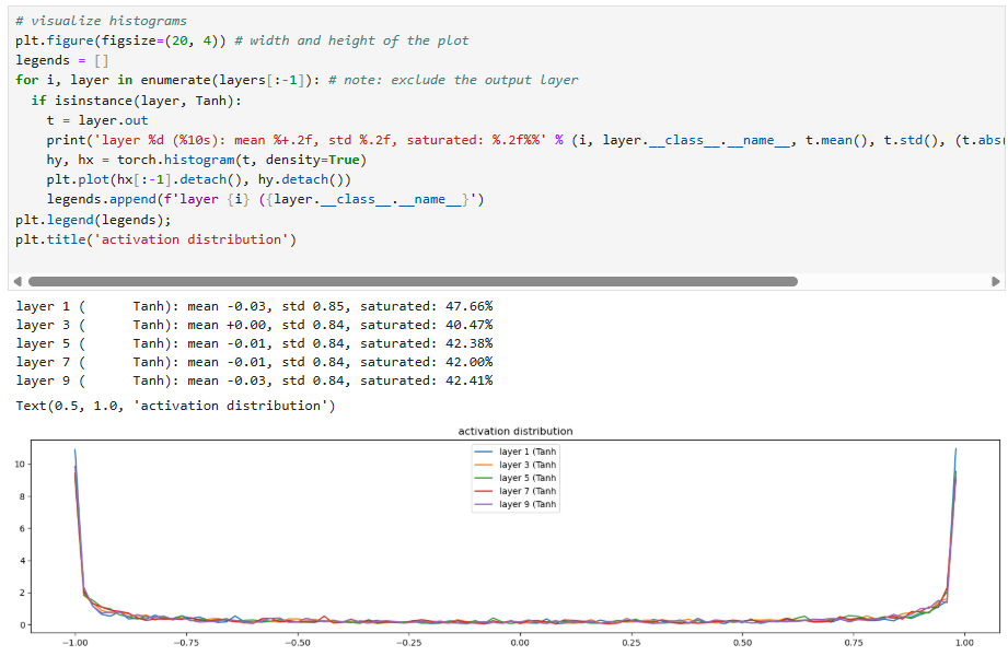
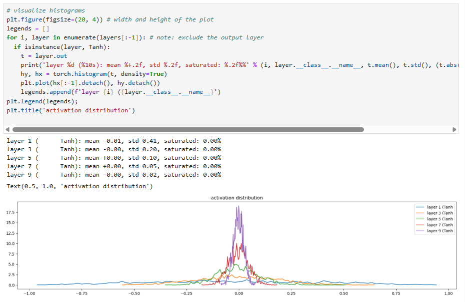
If we keep the gain as 5/3, as we saw from the PyTorch recommended gain for tanh:

The activations are:

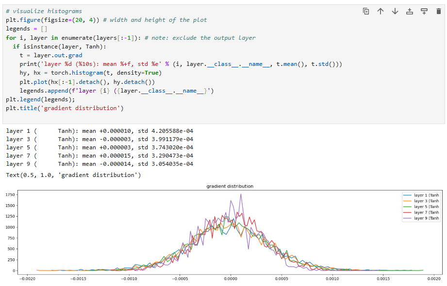
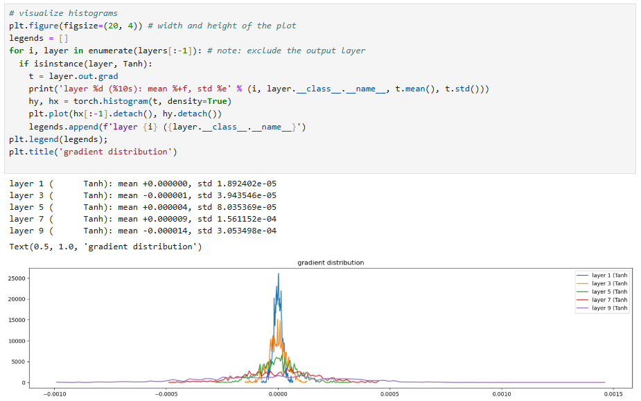
The gradients are:

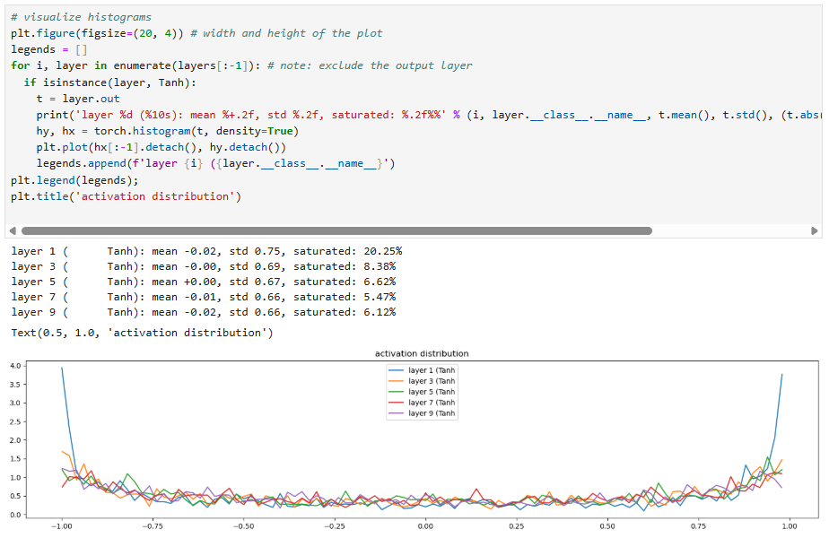
This shows that, before the use of batch normalization layers, neural network architects had to manually look at these plots to ensure that for each layer the activations are good in the forward pass (not exploding or shrinking) and the gradients looked good in the backward pass (again, not exploding or shrinking).

Here are some other diagnostic tools to make sure your neural network is training properly:

The below two images occur after 1000 training cycles:

Some more information about the weight matrixes, including the grad:data ratio

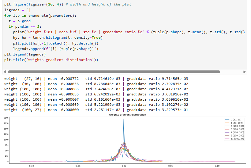
We see a problem: the standard deviation of the last layer's weight gradient is 10 times larger than the other layers' gradients. This means we are training the last layer 10 times faster than the other layers. This actually fixes itself, but this graph shows how even if the activation and gradients look okay, there is a lot of statistics to look at to make sure the neural network training is going okay.

Let's look at the update (lr * grad) to activation ratio as we train the neural net:

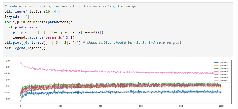
The last layer is an outlier because we artificially set the logits to be very low to make the predictions less confident. Here is the code proof for that:

with torch.no_grad():
  # last layer: make less confident
  layers[-1].weight *= 0.1
  # all other layers: apply gain
  for layer in layers[:-1]:
    if isinstance(layer, Linear):
      layer.weight *= 5/3
            

This can also help us set the learning rate. If the learning rate is too low, the rate of learning will be much lower, but if the learning rate is set to be too high, the rate of learning will appear to be far above the benchmark of 1e-3.

Let’s add BatchNorm to the PyTorch-ified code!

Let's now introduce batch normalization, so that we don't really need to worry about gain setting.

Here are the changes:

C = torch.randn((vocab_size, n_embd),            generator=g)
layers = [
  Linear(n_embd * block_size, n_hidden, bias=False), BatchNorm1d(n_hidden), Tanh(),
  Linear(           n_hidden, n_hidden, bias=False), BatchNorm1d(n_hidden), Tanh(),
  Linear(           n_hidden, n_hidden, bias=False), BatchNorm1d(n_hidden), Tanh(),
  Linear(           n_hidden, n_hidden, bias=False), BatchNorm1d(n_hidden), Tanh(),
  Linear(           n_hidden, n_hidden, bias=False), BatchNorm1d(n_hidden), Tanh(),
  Linear(           n_hidden, vocab_size, bias=False), BatchNorm1d(vocab_size),
]
# layers = [
#   Linear(n_embd * block_size, n_hidden), Tanh(),
#   Linear(           n_hidden, n_hidden), Tanh(),
#   Linear(           n_hidden, n_hidden), Tanh(),
#   Linear(           n_hidden, n_hidden), Tanh(),
#   Linear(           n_hidden, n_hidden), Tanh(),
#   Linear(           n_hidden, vocab_size),
# ]



with torch.no_grad():
  # last layer: make less confident
  layers[-1].gamma *= 0.1
  # layers[-1].weight *= 0.1
  # all other layers: apply gain
  for layer in layers[:-1]:
    if isinstance(layer, Linear):
      layer.weight *= 5/3
            

Remember, gamma now controls the spread of the softmax, so if we want to make the last layer's predictions less confident, we should change the gamma (like above).

By adding these BatchNorm layers, the activation and gradient of the nonlinearities, and the grad:data ratios for the weights are pretty robust to changing the gain value. However, the update:data ratio is still affected, so we need to pay attention to the gain when initializing our data values (or retune the learning rate if you change the gain).

TLDR: with batch norm we are a lot more robust to the gain and normalizing to the 1 / sqrt fan in and the grad:data for weights, but we do need to worry about the update:data ratio and tweak the learning rate accordingly

Summary of blog post:

• An introduction to batch normalization, one of the first modern solutions that help stabilize the training of very deep neural networks.
• How to PyTorch-ify our model (Linear class, BatchNorm1D, Tanh modules).
• Diagnostic tools to check if the neural network is in a good state:
• Stats histogram of the forward pass activations.
• Stats histogram of the backward pass gradients.
• Weights and how they are going to be updated - mean of grad, stddev of grad, and ratio of grad:data.
• Weights and how they are going to be updated - ratio of update (lr * grad):data over time.